How to Link Cells in Excel

Linking Cells in Excel is one of the most useful ways to create a direct reference between cells in your spreadsheets.

When you link one cell with another, the effect applies to both cells.

The best part is Excel allows you to link cells of the same worksheet, a different worksheet, and a different workbook. So, learn how to link cells from this article.

Using Paste Link Command

Firstly, you could use the Paste Link command to link two cells together in Excel. This method is pretty simple as we will Copy and Paste the value as usual. But, here, the Paste Link will just create a reference to the original source instead of copying the information. In this approach, you can link cell ranges within the same sheet or different sheets.

1. Select the cell or range. Then, enter the Ctrl + C to copy them.
2. Then, right-click on a new cell. Under Paste Options, click on Paste Special.
   
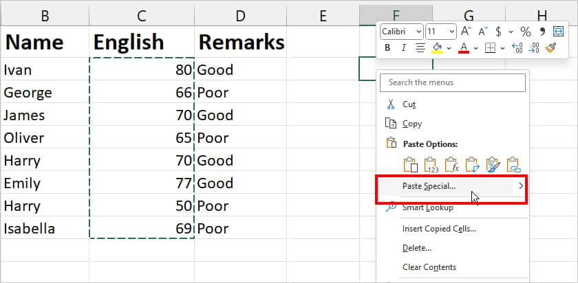
3. Click Paste Link.
   

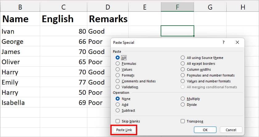
Now, when you edit the value of Column C, it’ll return the same changes in Column F too.

Create a Cell Reference

Another quickest way to link cells in Excel is to create a cell reference. I usually prefer this method because I can reference the cell ranges of different workbooks with just a single formula. Check out these 5 different cases to link cells.

Case 1: Link Single Cell

If you need to reference a single cell, simply enter =Cell Reference to return the same value in a new cell.

For example, if I enter =C4, it returns the value of the C4 which is 80 in a new cell. Similarly, when I change the value to 50, it’ll return 50 in the E2 cell too. 

Case 2: Link Cell Ranges Within the Same Sheet

To create a reference of Cell Ranges within the same sheet, here, we will use =Cell Ranges formula. 

For Instance, to link cell ranges from C2 through C5, type the formula mentioned in the box and press down Ctrl + Shift + Enter keys together.

=C2:C5

Case 3: Link Named Cell Ranges

It’s even easier to create a cell reference of ranges if you have named the ranges. You’d just have to enter =Named Range formula.

Let’s say, I have cell ranges from A2:A4, named Country. To link it, I’ll enter the formula as

=Country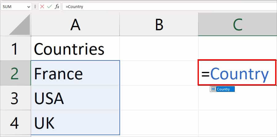

Case 4: Link Cells of a Different Worksheet

You can also create a reference of cells between two different worksheets in the same workbook. Just like other cell references, Excel will automatically update changes when you edit values in cells.

Here, you need to add a sheet name and cell range to the formula which would look something like this

=(Your Sheet Name)!(Cell ranges)

Let’s suppose, you need to link the value of cell C5 from Sheet 15 to a new Sheet. For this, your formula would be

=Sheet15!C5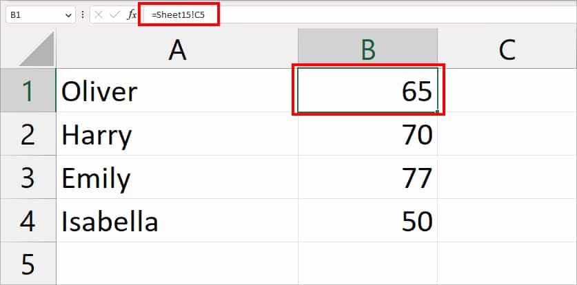

To avoid typos, use this method to input the references in the formula.

• Firstly, on a new sheet, enter = in a cell.
• Go to the Source sheet and select Cell reference.
• Press Enter to link cells.
• Then, extend the Flash-Fill if you want to reference multiple cell ranges from the source sheet. Note that while you use Flash-fill, Excel will return 0 in your new sheet if there are blank cells in the Original Sheet.

Case 5: Link Cells of Different Workbooks

If you want to link cells of different workbooks, we will create a reference using the workbook name, sheet name, and cell range in the formula.

='[(name of workbook).xlsx](sheet name)'!(referenced cell/range)

Suppose, you need to link the value of B2 through C7 from Sheet 14 of the Median workbook. For this, your formula would be

=[Median.xlsx]Sheet14!$B$2:$C$7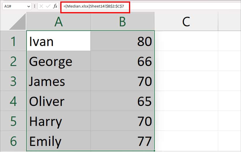

Again, use the same trick as above instead of entering the formula manually. This way you can ensure the cell references are correct.

• Firstly, Open both workbooks.
• Then, in a new cell of the destination workbook, enter =.
• Head to the Source workbook and select Cell ranges from the worksheet.
• When done, press Enter.

Create 3-D Reference

In Excel, when you create a reference of the same cell of multiple worksheets, it refers to a 3-D reference. For Instance, if you link C2:C5 cell ranges of both Sheet 14 and Sheet 15, it is a 3-D reference. 

Moreover, you can also use VSTACK, SUM, PRODUCT, MIN, MAX, and many more functions to create a 3-D Reference.

Here, we will cover the example for SUM 3-D reference. This type of reference sums up the total values of cell ranges. So, if you want to merge the values of different sheets, this method is for you. When you modify the numbers in any one of the sheets, your total output also changes.

To create a Sum 3-D reference, we will use the SUM function in the formula. Suppose, you need to calculate the total output of C2:C5 ranges from Sheets 14 and 15. For this, use the formula mentioned in the box.

=SUM(Sheet14:Sheet15!C2:C5)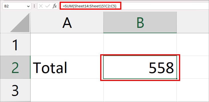

Follow these steps to input the formula in the cell.

1. On a new sheet, enter =SUM(
2. Head to Sheet 14 and select C2:C5 cell ranges.
3. While holding the Shift button, select Sheet 15.
4. Press Enter.