How to Ignore All Errors in Excel? 5 Easy Ways

While working on Excel, you might commonly encounter errors like #DIV/0, #N/A, #NAME?, #NULL!, #NUM!, #REF! and #VALUE!, generally indicated with a green triangle in the top-left corner of the cell. There are a number of reasons why Excel might trigger these errors, some of the more probable reasons being:

• #DIV/0! Error: When you divide a number by zero or an empty cell.
• #N/A Error: When Excel cannot find the value you want.
• #NAME? Error: When Excel does not recognize a formula name or a named range.
• #NULL! Error: When you use a space instead of a comma to separate arguments in a formula.
• #NUM! Error: When you use an invalid argument in a formula.
• #REF! Error: When referencing an invalid cell or range in a formula.
• #VALUE! Error: When you use an invalid data type in a formula, such as text instead of numbers.

There are times when you want to ignore those errors and move on with your work. While ignoring these errors should not be your first option, you might need to avoid them when you’re yet to finish data entry or are creating a template. For such situations, Excel has a list of tools and functions to ignore certain errors.

Use Ignore Error Option

Excel allows you to ignore the error and hide the error indicator using the Ignore Error option.

For example, if you try to divide a number by zero, Excel will throw out an error #DIV/0. You can ignore errors like this and several other errors in Excel using the Ignore Error option. 

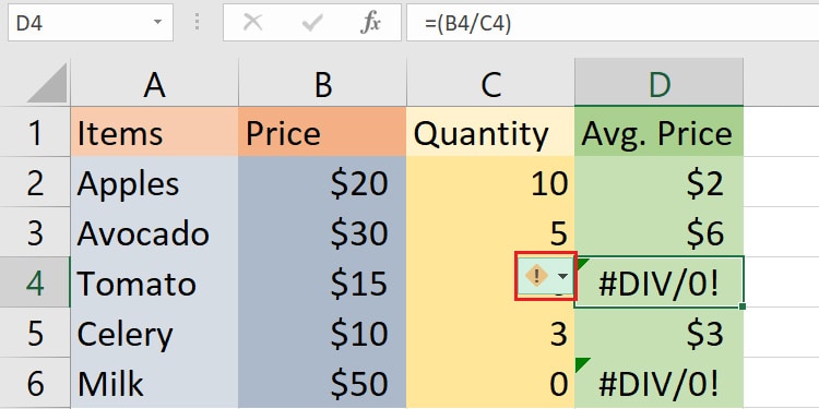
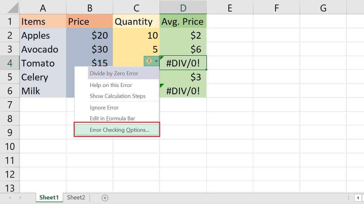
You can see that there is an #DIV/0! error in D4 and D6 cells. I’ll try to ignore this using the same option.

1. Open the Excel Spreadsheet.
2. Hover on the error indicator next to the cell with the error message.
   
3. Select the columns where you want to remove the errors.
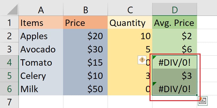
4. Hover over to the error indicator and click on the drop-down menu.
5. Click Ignore Error to ignore errors from the entire column.

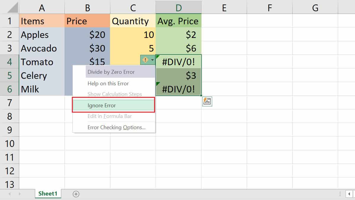
This option allows you to ignore all sorts of errors but is limited to a single cell and a column. If there are too many errors in your worksheet and you want to ignore errors in the entire sheet, you may consider the next method.

Disable Error Checking Option

Another easy way to ignore all the errors is to turn off the error-checking feature in Excel. Turning off the error checking will remove all the errors and make your spreadsheet look error-free.

To implement this option, I’ll use the above example of groceries item and ignore all errors simultaneously.

1. Open the Spreadsheet and hover on the trace error indicator.
2. Click the drop-down menu and select Error Checking Options.
3. Uncheck the Enable Background Error Checking, and hit Ok.

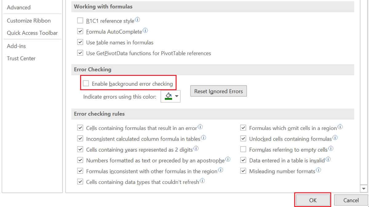
Turning off the error-checking option will ignore all the errors in the Excel spreadsheet, so sometimes you might be unaware of the data that needs to be corrected.

In such a case, you can uncheck the rules that you don’t want to enable under the Error-checking rules section.

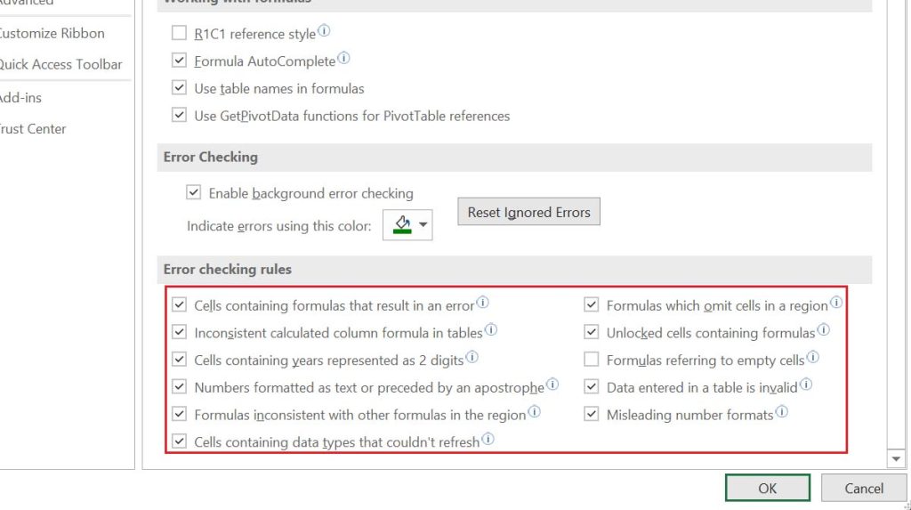
You can now create your own rules by selecting the rules you want to add, and it will only ignore those selected errors.

Using the IFERROR Function

Another way to ignore errors in Excel is the error-handling functions. These functions allow you to test for different types of errors and return a value or formula accordingly.

The IFERROR function is one error-handling function that hides your error message from the spreadsheet.

Syntax: =IFERROR(value, “value_if_error”)

Here,

• Value: A value, reference, or formula to check an error.
• Value_if_error: It is the value to return if an error is found.

Using this function in Excel, you can replace the error message with your custom message when there is an error. 

Example:

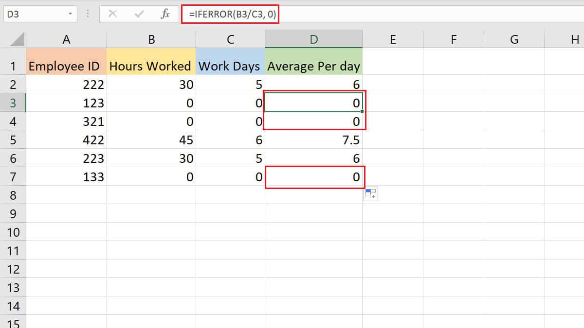
Let’s say a company has a record of all employees—their total working hours and work days. Now, here is a spreadsheet to find the average working hour of each employee.

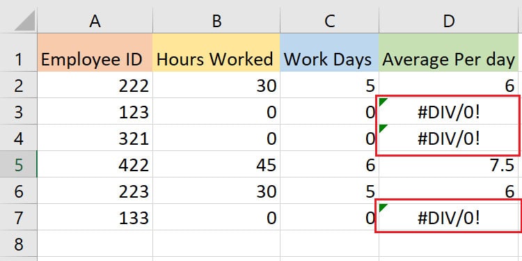
Excel throws a #DIV/0! error in D3, D4, and D7 cells when I directly divide the hours worked by work day to find the average working hour.

However, you can see that I use the IFERROR function to replace the errors with “0.”

Using the ISERROR Function

You can use the ISERROR function in Excel to check if a cell or formula contains any error. It will return TRUE if the value is an error and FALSE otherwise.

You can use the ISERROR function to ignore the error when Excel cannot calculate or find a value.

Syntax: =ISERROR(Value)

You can also use the ISERROR function with the IF function, displaying a custom message instead of TRUE or FALSE. 

Example:

Suppose we need to determine the price per unit of the item you bought. When I use the formula directly to find the price of an item per unit, there is a #VALUE! error in D4 cell and #DIV/0! error in D5 cell.

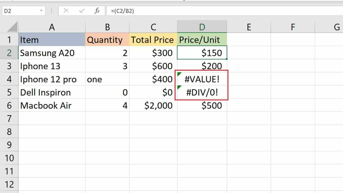
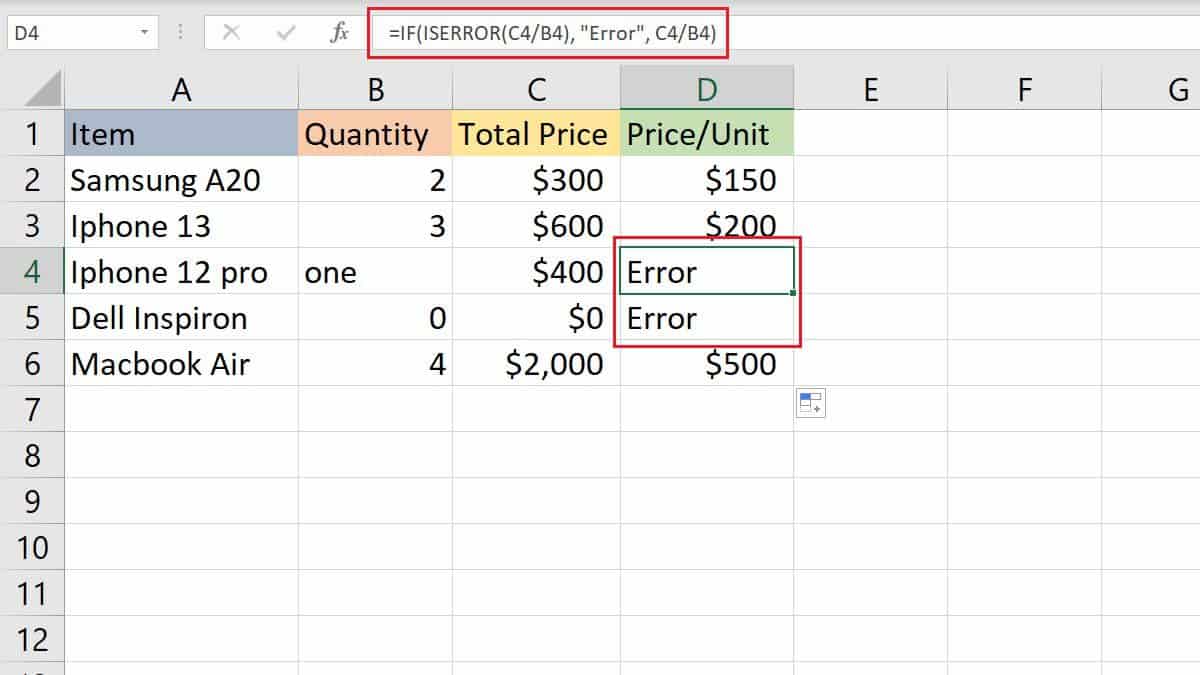
Now, I will try to ignore these errors using the ISERROR function. Here, I will use the ISERROR function with the IF function to show a custom message instead of a TRUE or FALSE value.

Instead of the error, a custom “Error” message is displayed when I use the ISERROR function.

Using IFNA Function to Ignore #N/A Error

You can use the IFNA function in Excel specifically to ignore the #N/A error. This error in Excel represents a “no value available” error in the output.

Syntax: =IFNA(value, value_if_na)

Here,

• Value: A value, reference, or formula to check #N/A error.
• Value_if_na: It is the value to return if a #N/A error is found.

Example:

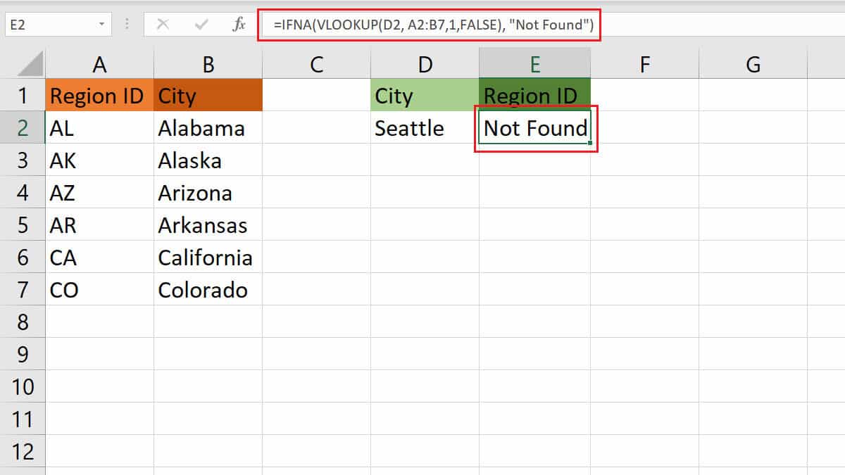
In the spreadsheet below, different cities and their corresponding region IDs exist. We want to find the region ID of a specific city using the VLOOKUP function. However, there is an #N/A error in the E1 cell when you place a city name not in the datasheet.

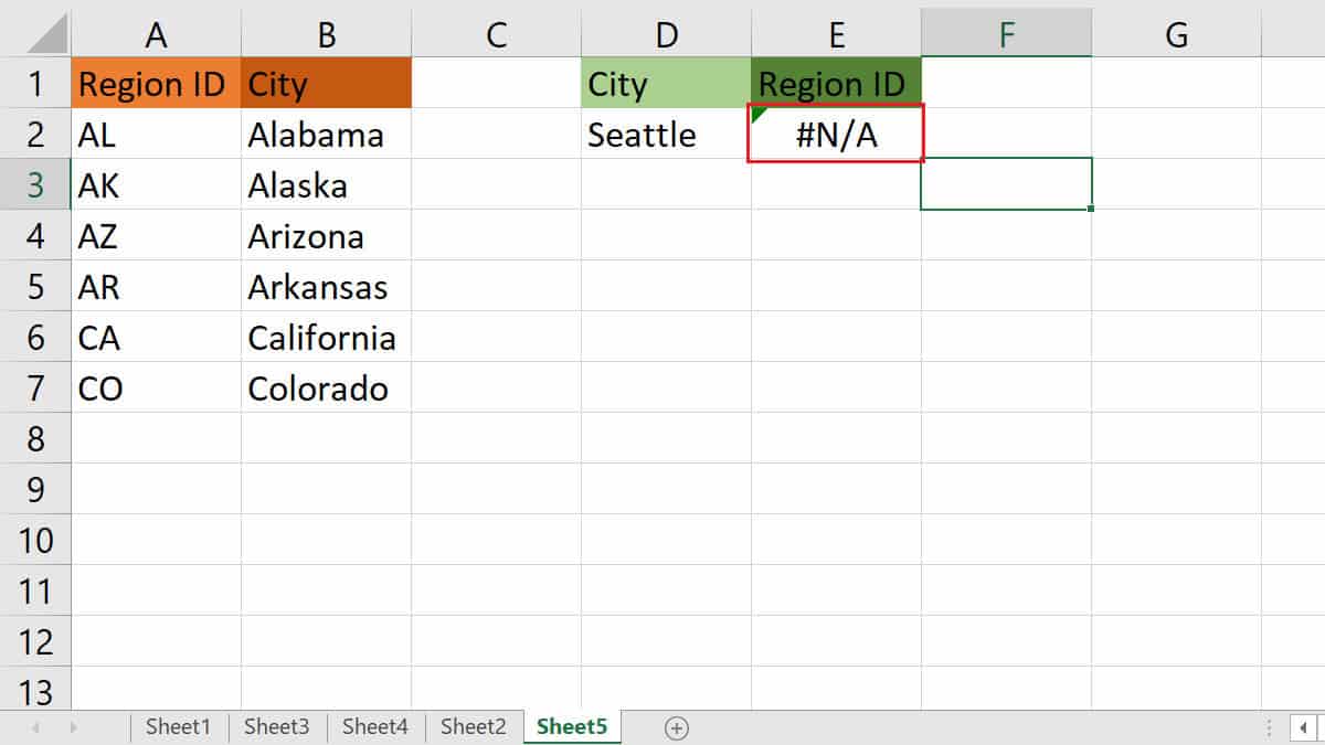
You can use the IFNA function to ignore this #N/A error from the VLOOKUP function.

Here is the result when I use the IFNA function to ignore the #N/A error message in my spreadsheet with a custom “Not Found” message.