How to Hide Columns in Google Sheets

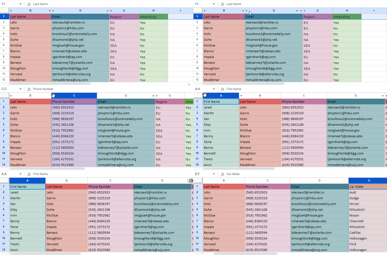
Working in Google Sheets can get tedious when you are have a large data set.

Let’s assume your worksheet contains 15 columns. All of those columns will not fit on your screen, and you will have to keep scrolling back and forth if you are working with columns that are far apart. 

In such scenarios, Google Sheets has a user-friendly feature to hide columns to ease your work. It allows you to hide specific columns from your worksheet to compare few distant cells or even print specific cells from the worksheet. 

With Right-Click Option 

The hiding column option can be hard to spot if it is your first time. But once you’ve spotted it, you’ll realize how quick and easy it is.

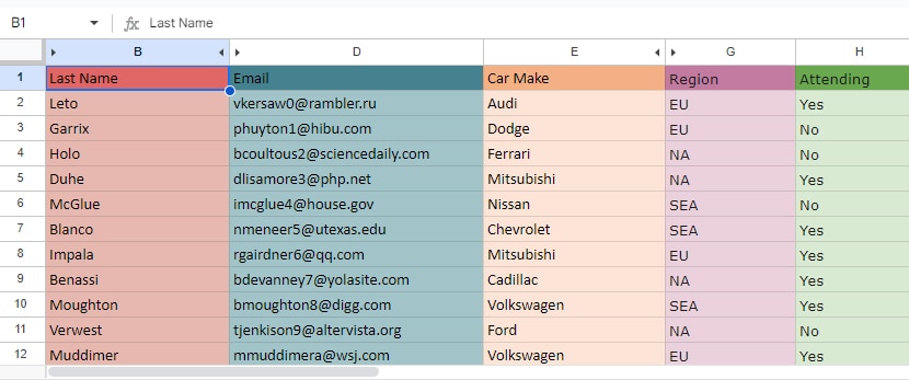
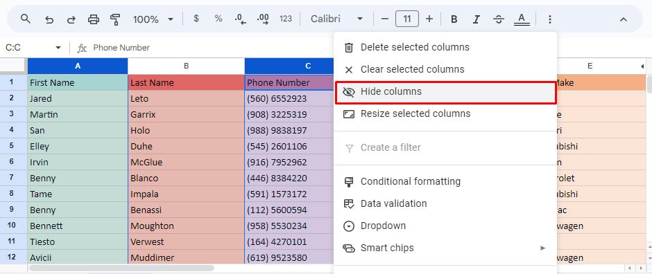
To hide a certain column, first select the column. Then, right-click and select Hide Column.

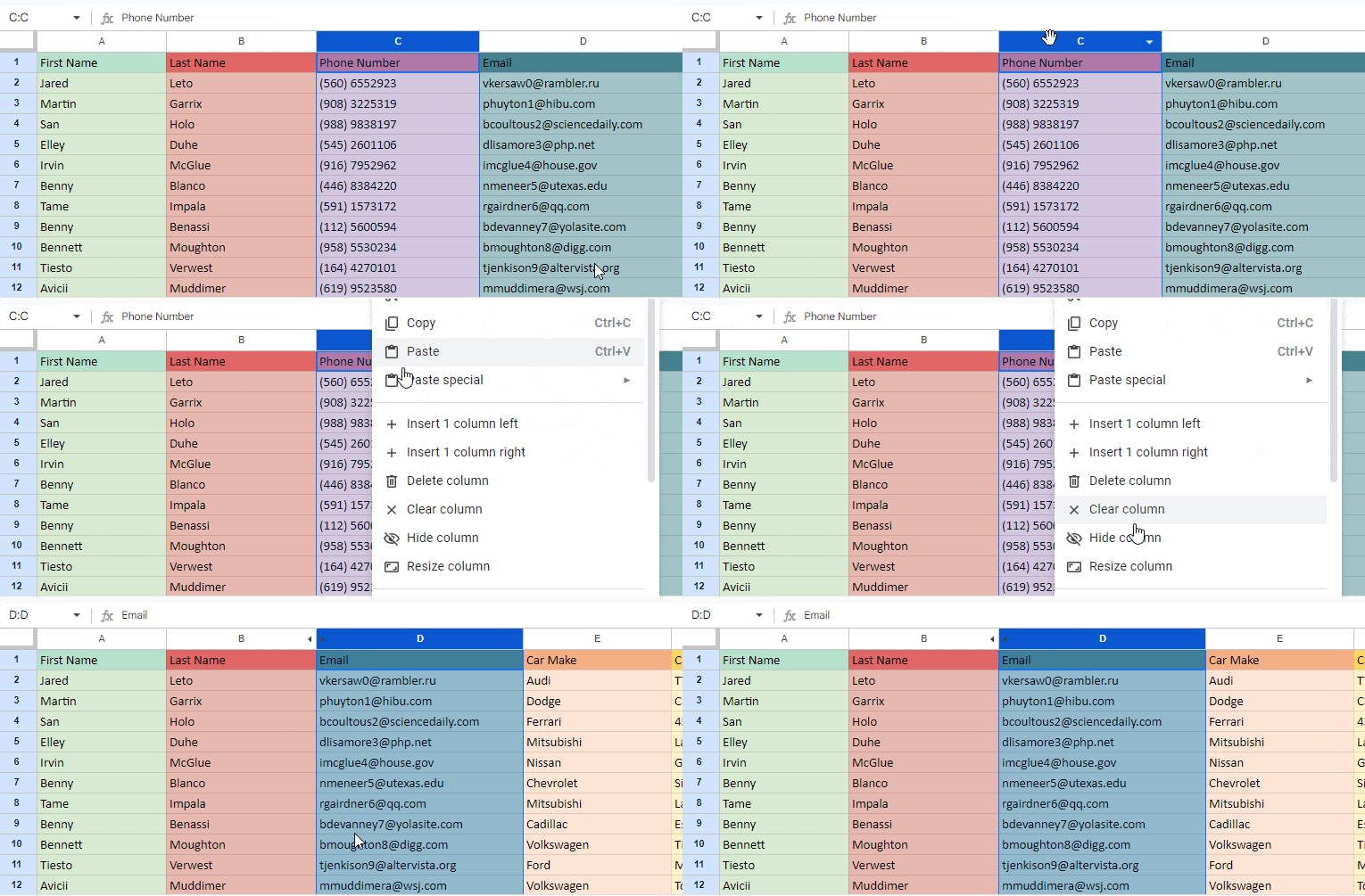
To hide multiple columns, hold the CTRL Key and select the columns you want to hide. Now, right-click on any column heading and select Hide Column.

With Keyboard Shortcut Option

If you want another way around hiding columns on your Google Worksheet, you can use a keyboard shortcut as well.

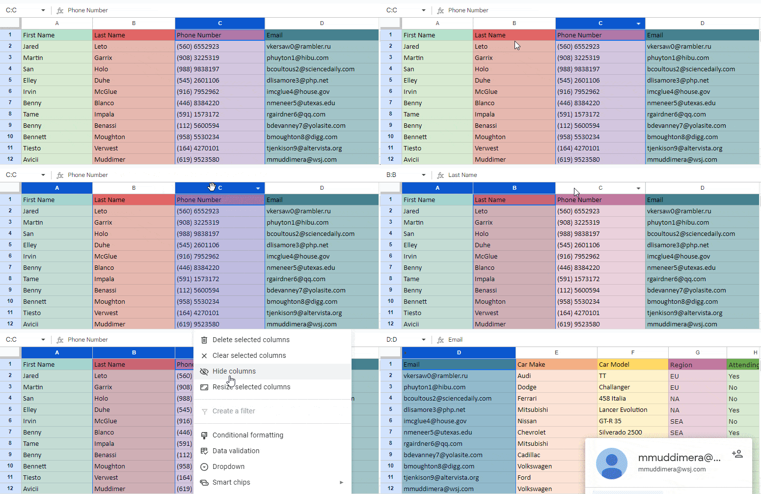
To hide any column using the keyboard shortcut, first select the column you want to hide. If you want to hide multiple columns, hold CTRL on your keyboard and select the column headings.

Then press CTRL + ALT + 0 on your keyboard.

How to Hide Columns in Google Sheets From Certain Users?

Google Sheets also provides the option to protect columns, meaning you can lock specific cells and choose whom you want to grant access to view the protected columns. This way, the columns are hidden and you can restrict specific users from viewing the details of the protected columns.

Here are the steps to protect and hide columns from users.

1. Right-click on the column you want to lock.
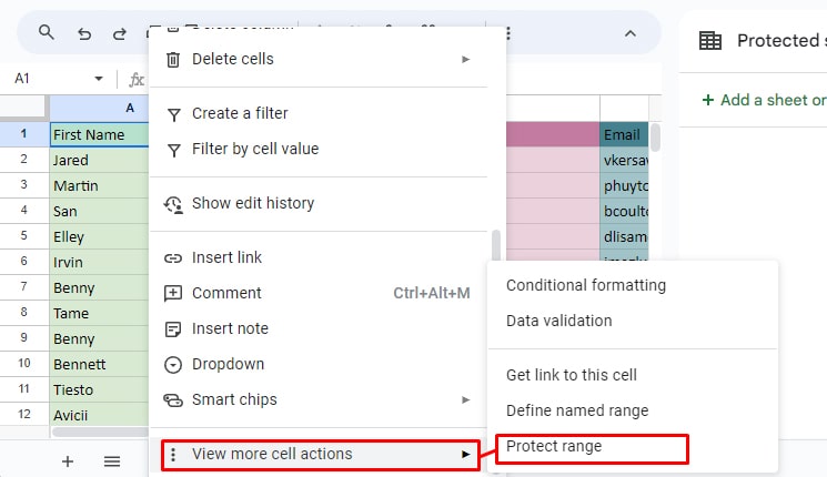
2. Navigate down to View more column actions > Protect Range.
   
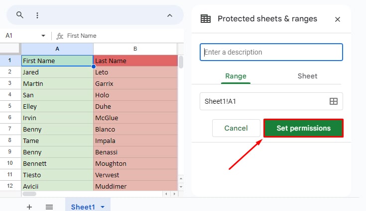
3. Click on Set Permission. 
   
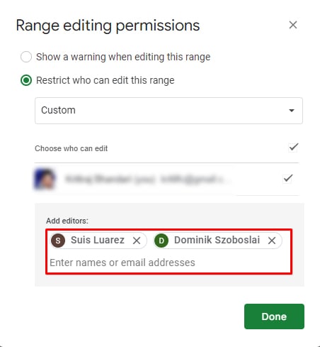
4. Go to Custom if you want to set range editing permission.
   
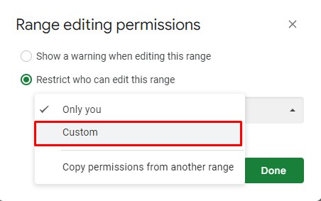
5. Grant editor access to users whom you want to allow editing on the Sheets and Click Done. 
   

Alternatively, if you want to share only specific information from your datasheet, then you can hide the columns and share the sheet with other users. However, you need to set the access to Viewer.

If you set the role to the editor, then the user with the link will be able to unhide the columns.

Here is how you can do it:

1. Select the column you want to hide.
   
2. Right-click on it and click on Hide Column. 
   
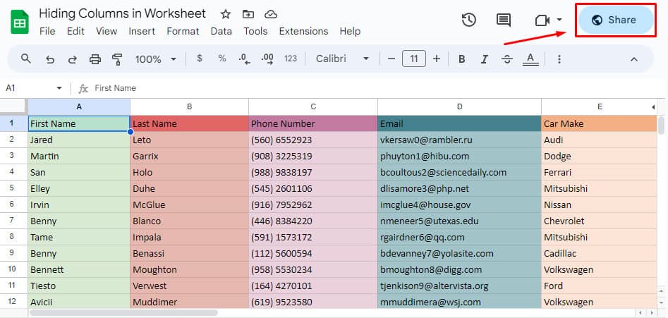
3. Click on Share.
   
4. Under General Access, click on Anyone with the link. 
   
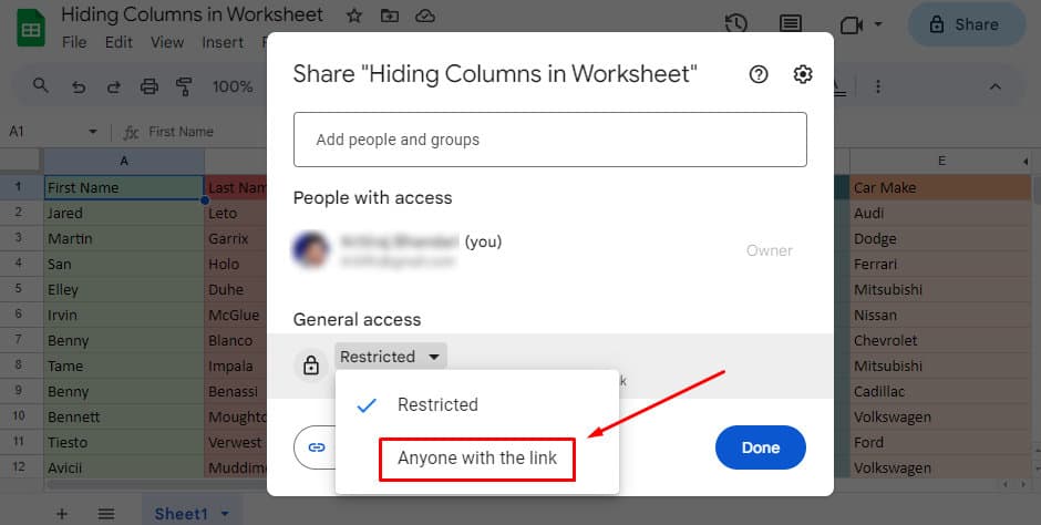
5. Set the role to Viewer and click on Done. 
   

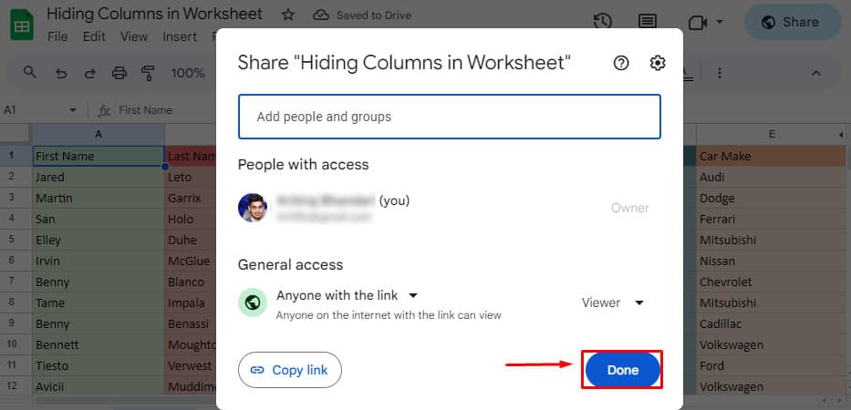
Now, the hidden columns won’t be visible to the shared people/group. 

Unhiding Columns in Google Sheets

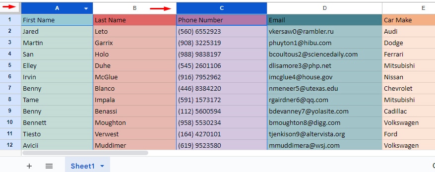
Your hidden columns can be spotted in the column headers section. If you find that the column headers are not in chronological order, then that means the columns have been hidden. To unhide the columns, follow these steps.

1. Open Google Sheet.
2. Spot the following sign to locate the missing cells. 
   
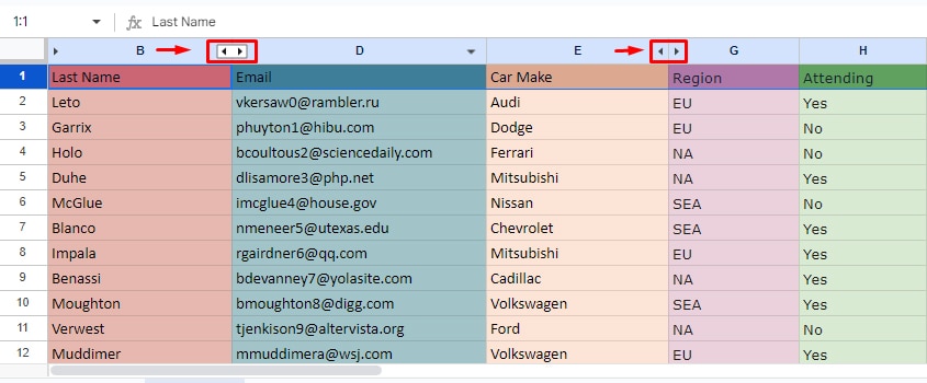
3. Click on the icon to unhide the columns.