How to Group Cells in Excel

While calculating subtotals, you’ll have lists of identical values displayed under one heading in your sheet. But, do you want to keep all of them in view?

Well, if you group the same rows or columns, you can use the Outline Symbols (+) and (-) to hide/show ranges.

Let’s take, for instance, you can choose to display only the Subtotals of the Product named “Speaker” and hide the remaining information. This way, your sheet would look more clean and organized, isn’t it?

Using Group Menu

In Excel’s Data tab, you can find the default Group menu to group rows and columns. You can manually group multiple cell ranges or use an auto-outline to quickly create groups. 

Step 1: Group Rows or Columns

1. On your sheet, select Cell ranges.
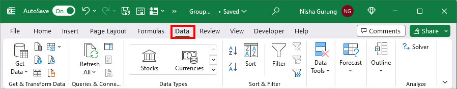
2. Go to Data Tab.
   
3. In the Outline section, expand the drop-down menu for Group. Then, choose one of the following:
   
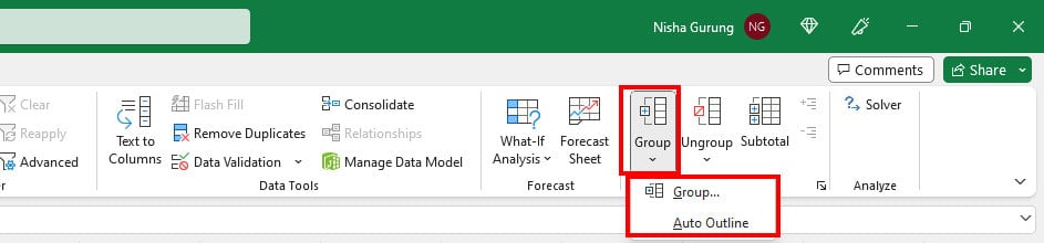
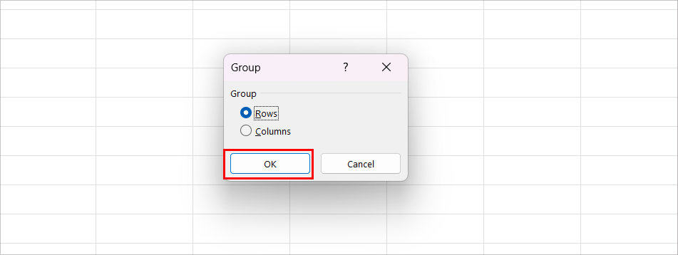
   • Group: Manually group rows and columns. This option is best if you want to nest grouped ranges. If you pick this option, click on either Rows or Columns in the Group window and click OK.
     
   • Auto Outline: Once you click this option, Excel will auto-group the rows and columns based on your summary or subtotal.

Alternatively, there’s also a keyboard shortcut to group cells manually in Excel. Though the shortcut begins with the Alt key, it isn’t a ribbon shortcut. Meaning, you need to press all the keys together. 

Keyboard Shortcut: Alt + Shift + Right Arrow Key

After you press the keys, a Group window will appear on your screen. Pick either Rows or Columns. Then, hit OK.

Step 2: Collapse/Expand Grouped Data

Now, that you have grouped the rows or columns, you will see an outline on the left side of your sheet. It displays outline symbols like (1, 2, 3) and (+, -) to show or hide the ranges. 

If you want to collapse the rows/columns based on the levels, click on numbers (1, 2, 3). In our example, 1 shows only Grand Total, 2 keeps all the Subtotals in view, and 3 displays everything.

But, if you wish to collapse a specific grouped range, click on the – sign. When you do this, it’ll only show the subtotals. Likewise, to expand the hidden items again, click on the + icon.

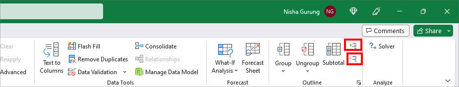
Apart from Outlines, you can also perform these actions from the Excel Ribbon. Head to the Outline group in Data Tab. Then, click on the Hide Detail menu to collapse the grouped ranges or select the Show Detail icon to display them again. 

Step 3: Customize Outline Style

To make your grouped data look more presentable, you can apply automatic styles after creating the outline.

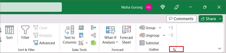
1. Go to Data Tab.
2. In the Outline section, click on the Dialogue Box Launcher for Advanced menu.
   
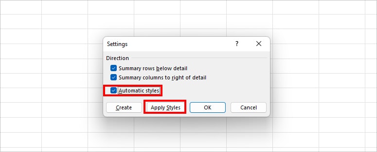
3. On the Settings window, tick the box for Automatic Styles and click Apply Styles.
   

Using Subtotal Feature

Let’s say you have identical data and wish to group the rows. But, there are no subtotal values in your range. During such instances, you can use the Subtotal tool to group ranges, return the subtotal, and grand total values all at once. Besides, this tool is also useful when you want to calculate the subtotal of products, average, max, etc.

1. On your worksheet, select all Data.
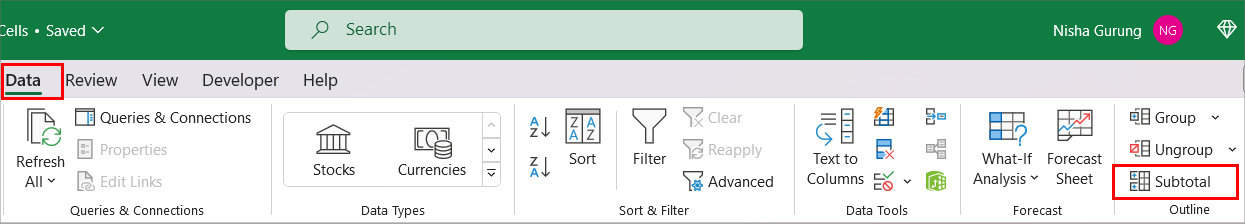
2. Go to Data Tab. In the Outline section, click the Subtotal.
   
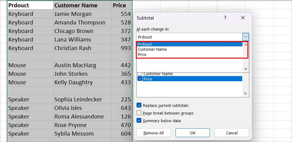
3. On the Subtotal window, expand the drop-down menu for At each change in and choose a Column.
   
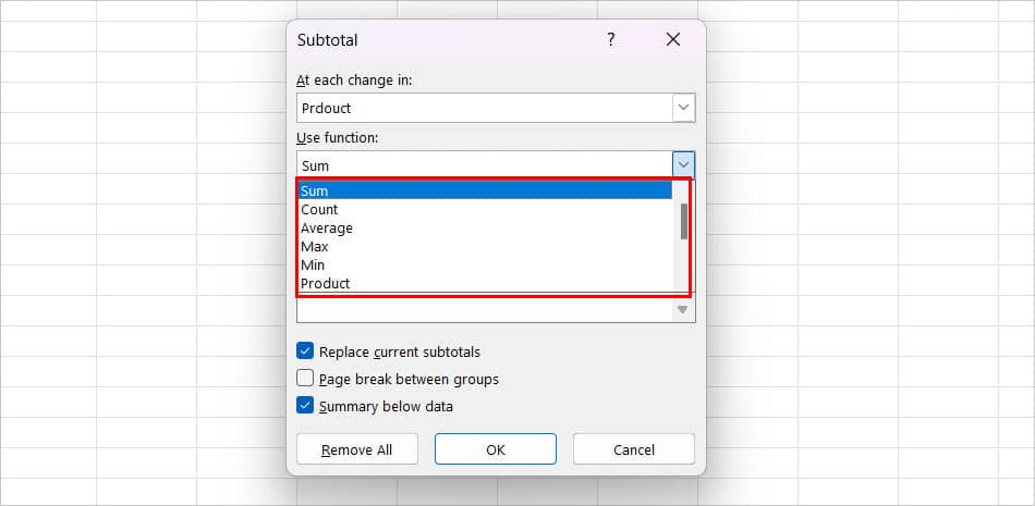
4. Below Use function, pick a Function to return the value in. For example, if you choose Sum, it’ll return subtotal.
   
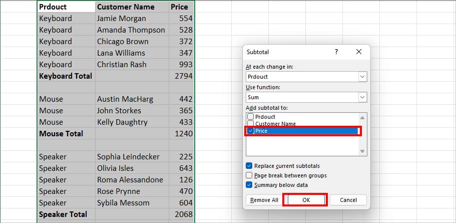
5. Under Add subtotal to, tick the boxes for the Column Name to insert Subtotal. Then, click OK.
   
6. Now, use the 1, 2, 3 outlines to display each level of grouped data.
   
7. If you want to hide/unhide certain grouped ranges manually, click on the (-) and (+) icon.
   

Using Pivot Table

Just like the Group and the Subtotal menu, Excel’s Pivot Table is also used to summarize similar values under one header. When you create a Pivot Table, you’ll automatically have subtotals and grand totals for the values. Moreover, you can also filter the values and choose to show only the required information at a time. So, how is it so different from the rest two methods? 

Since Pivot Tables are dynamic, you can simply refresh the table to update the values from your source sheet/range. 

1. Click any Cell within the Table/Data.
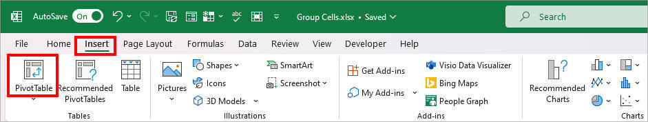
2. Go to Insert Tab and click on PivotTable in the Tables section.
   
3. On the PivotTable window, choose the Table/Range using the collapse icon.
   
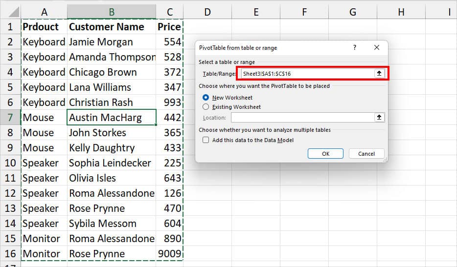
4. Below Choose where you want the PivotTable to be placed, pick one of the locations:
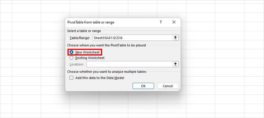
   1. New Worksheet: This option will create a Pivot Table in New Sheet.
      
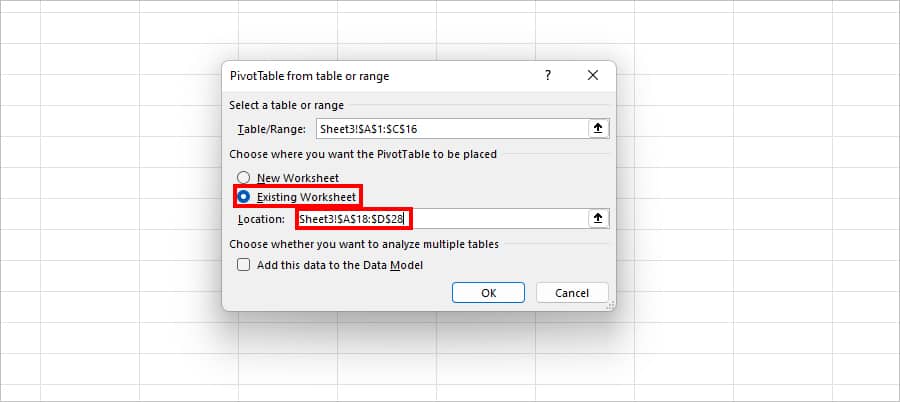
   2. Existing Worksheet: Insert Pivot Table somewhere in your Current Sheet. If you choose this, select a cell range with the Collapse icon.
5. Click OK.
6. Now, hover over the PivotTable Fields on the right side of your Sheet. Tick the boxes for the column headers you want to show.
   
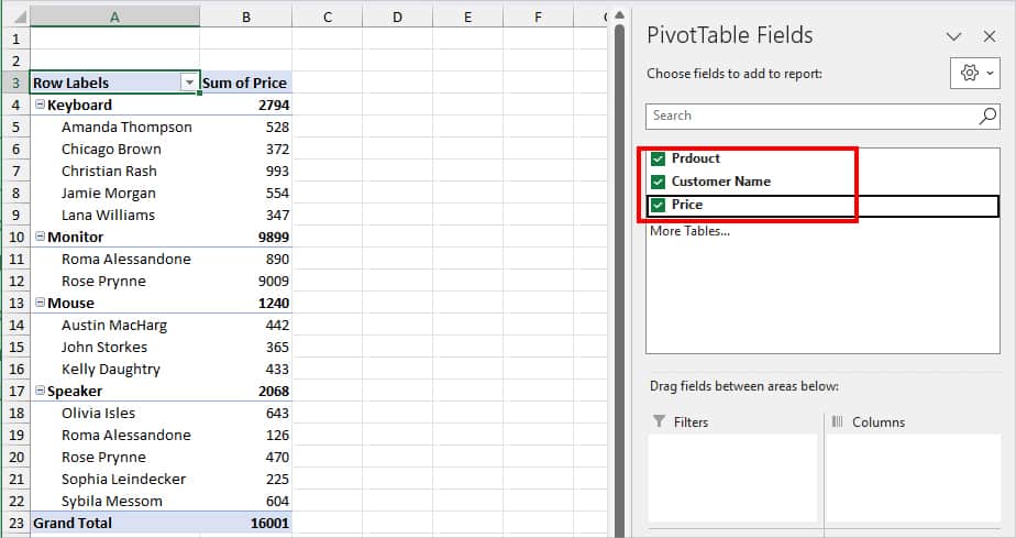
7. If you look into the Pivot Table, you can see a Minus icon (-) for each Row header. Click on the minus sign to collapse the sub-headings. Similarly, click the + symbol to expand the data.
   

Why can’t I see Outline Symbols for Grouped Data in Excel? 

I know it’s a lot quicker and simpler to just click on the Outline Symbols to hide/show your grouped data. After grouping ranges, you should immediately see these outline icons. But, if you do not see them, check your worksheet display options and add them.

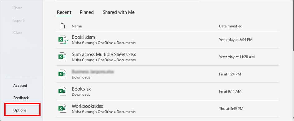
1. Open Excel.
2. Go to the bottom and click on Options.
   
3. Now, from the side menu, go to Advanced.
   
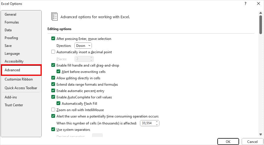
4. Scroll to find the Display options for this worksheet menu. Then, tick the box for Show outline symbols if an outline is applied.
   
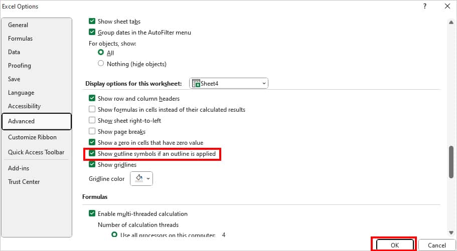
5. Click OK. 

How to Ungroup Cells in Excel?

If you wish to ungroup the rows/columns, you can find the default Ungroup menu in the Data Tab. This method is for users who have grouped cells using the Group or Subtotal menu. 

1. First of all, click on any cell with Outline. 
2. On Data Tab, click Ungroup and pick one of the following options.
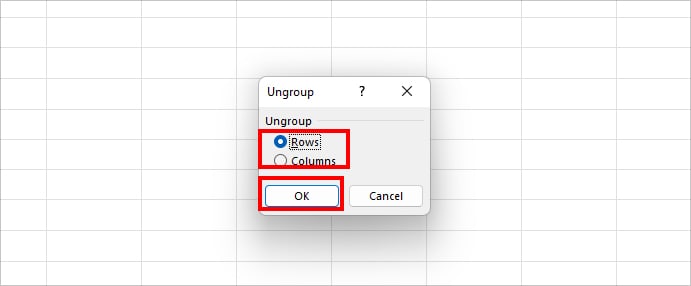
   1. Ungroup: Choose this to ungroup only certain Rows or Columns. In the Ungroup window, pick either Rows or Columns. Hit OK.
      
   2. Clear Outline: Immediately removes all Grouped outlines. 

In case you have Pivot Table, you could Unpivot Data to ungroup them.