In Excel, the more giant spreadsheet you have, the more number of rows and columns will be. If you have such a huge sheet, learning how to freeze multiple rows and columns is definitely the best idea.
You could keep a set of rows and columns locked while you’re scrolling the rest of the sheet. Eventually, data comparison becomes easier as you can view the desired information within your sheet at once. You wouldn’t have to scroll all the way up and down every time.
To freeze multiple rows or columns, there’s a menu called “Freeze Pane” in Excel. But, if you just want to view and not lock them, you could split the window instead.
Things You Need to Know Before Freezing Multiple Rows or Columns
- Your Active cell determines the number of rows and columns to freeze in the sheet. Meaning, Excel will freeze all the rows above from your active cell. Similarly, it locks all the left columns from the current selection.
- For Example, D7 is my active cell. If I freeze panes, Excel will lock Rows from 1 to 6 and A, B, C columns.
- Once you’ve frozen panes, you cannot use Ctrl + Z to Undo. You’d have to manually Unfreeze Panes.
- Excel does not allow you to lock Top Row, First Column, and Multiple rows together. You can only freeze one of them at a time.
How to Freeze Rows or Columns in Excel
Using Keyboard Shortcut
If you need to freeze multiple rows and columns in Excel regularly, I suggest you use the Keyboard Shortcut for this. With these shortcuts, you can instantly freeze and unfreeze panes in your sheet anytime.
To do so, click on a cell and enter the following keyboard shortcuts together. Note that when you enter keys, you do not have to press and hold them as you’d do for other shortcuts. Since this is an Excel ribbon shortcut, you can enter each key one after another. For Instance, press the Alt key. Then, enter W, F, and so on.
Shortcut key: Alt + W + F + FFrom Excel Ribbon
You can also freeze a set of rows and columns from Excel’s ribbon. If you do not prefer shortcuts to perform tasks, this method is for you. Here, you can find the default Freeze Panes menu to do so.
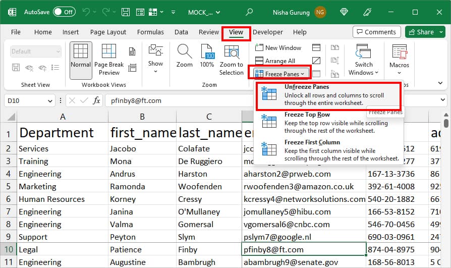
Firstly, select a cell on your spreadsheet and go to View Tab. From Window Section, click Freeze Panes > Freeze Panes.
From Quick Access Toolbar
You can add a number of individual commands in Excel’s Quick Access Toolbar to do tasks even more efficiently. As the name itself indicates, you can quickly access and use the added commands from the toolbar.
Here, we will insert the Free Pane command in the Quick Access Toolbar first. Then, we will click on the icon to use the command.
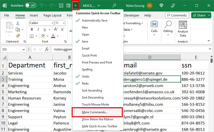
- Hover over Quick Access Toolbar.
- Expand the More icon > More Commands.
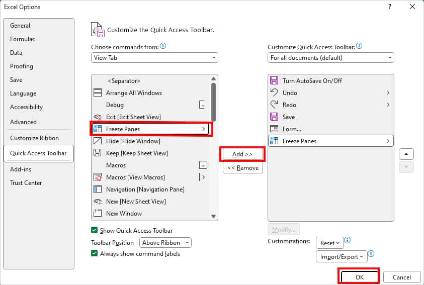
- On Choose commands from, pick View Tab.
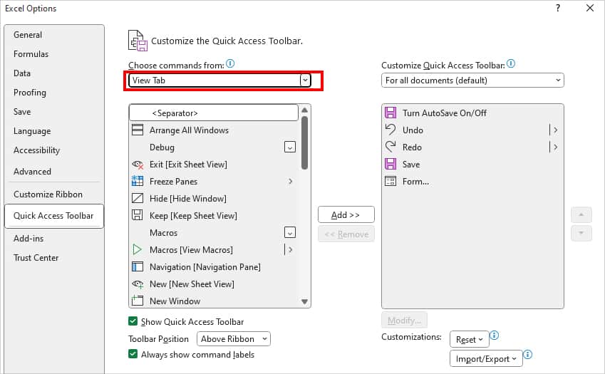
- Select Freeze Panes and click Add. Then, hit OK to confirm.
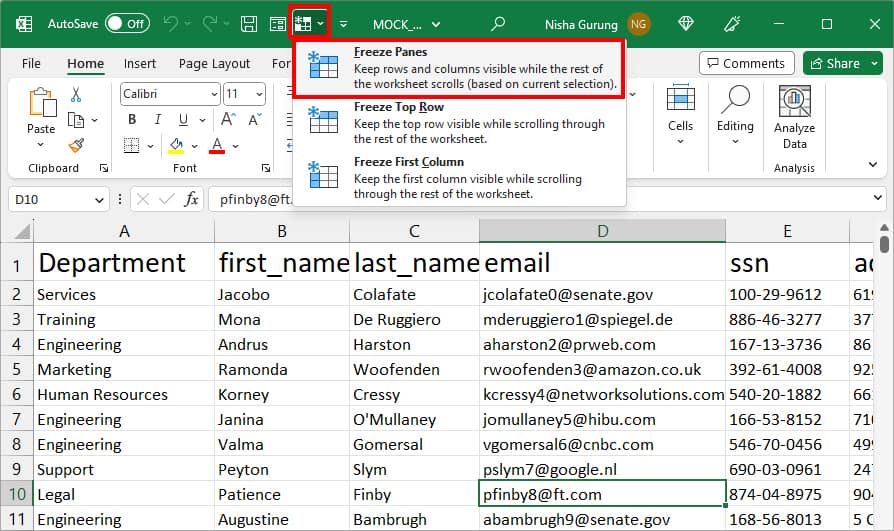
- Now, to freeze panes, select a cell. From Quick Access Toolbar, click on Freeze Panes Icon > Freeze Panes.
Split Window
Another way to freeze several Columns and Rows is by using the Split menu. As the Split menu is mostly used to view two parts of a sheet side by side, it is pretty much similar to freezing rows/columns.
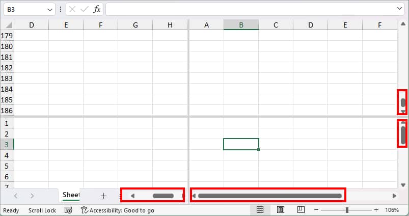
At first, the Split menu will freeze the above rows and left columns from your active cell. But, unlike the Freeze Pane, you can actually scroll through endless rows and columns in both split windows.
I especially prefer this method because the Split view displays two scroll bars for each window. So, I could just select the window and scroll the row or column separately at a time. The best part is it allows you to drag the Split line to re-adjust the rows or columns view.
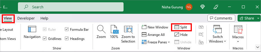
To split the sheet, all you need to do is select a Cell and go to the View Tab. From the Window group, click on Split.
Alternatively, there’s also a ribbon shortcut for this. Once you choose your active cell, enter the following keyboard shortcuts. The shortcut also works to turn off the Split View.
Shortcut key: Alt + W + SHow to Unfreeze Multiple Rows or Columns in Excel?
After you freeze the multiple panes, you cannot freeze Top Row or First Column along with it. To use these options, you’d have to unfreeze first.
The quickest way to unfreeze panes is by using the same shortcut key as above.
Keyboard Shortcut: Alt + W + F + FAlternatively, you can also unfreeze from Excel Ribbon. For this, head to View Tab. Click on Freeze Panes > Unfreeze Panes.