If you need to analyze the performance based on numbers, you’d definitely look for the highest and least value in Excel. Be it a sales report, golf scores, student mark sheet, and many more. Knowing the lowest number can help you determine the last position as well as make better decisions.
In Excel, you can not only find the least number but also highlight them. So, today, let us learn how to identify the minimum value from data in different circumstances. You can find 8 different methods to do so in this article.
Using Analyze Data
Did you know you could ask questions about your data in Excel and easily retrieve answers?
Excel’s “Analyze Data,” previously known as “Ideas in Excel” is built to make your data analysis process easier and quicker. So, let us determine the lowest number from your data with this amazing feature. Note that you must have Office 365 subscription to use this feature.
- Firstly, select your data ranges.
- From Home Tab, click on Analyze Data.

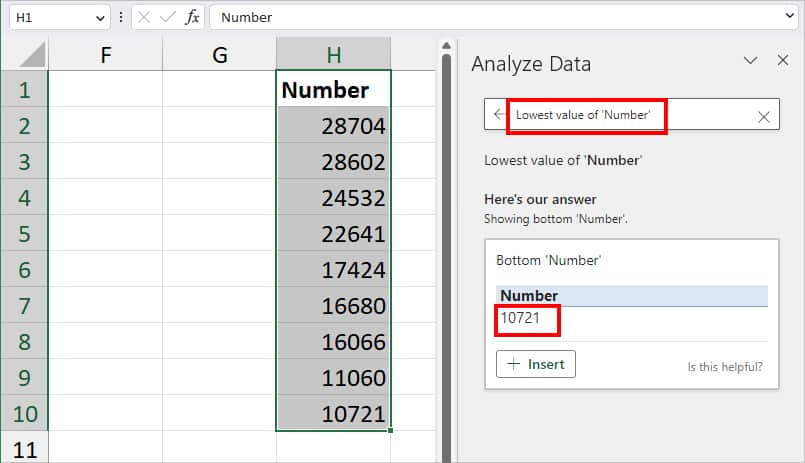
- On Analyze Data, enter the Lowest value in the search bar and click on Suggested Search. You can see the answer in the right panel.
Using Sort & Filter
Another fastest way to identify the smallest number in Excel is by re-arranging the values in the Smallest to Largest Order. If you have only numeric values without the linked information in the adjacent column, you can use the Filter button.
- Firstly, select the data and head to the Data Tab.

- From Sort & Filter, select the Filter menu to turn it on.

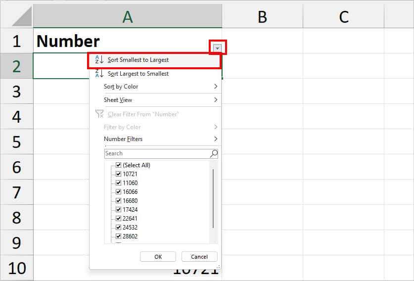
- Click on the Filter button and pick Sort Smallest to Largest.
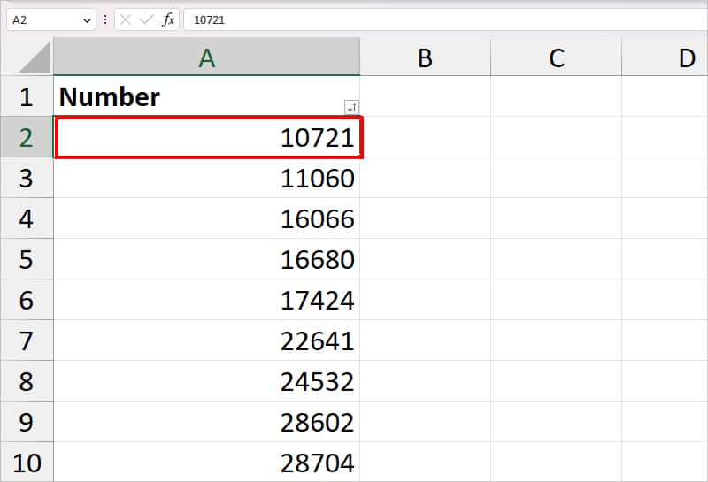
- Now, the smallest number will appear at the top.
Using the Bottom Rule of Conditional Formatting
Conditional Formatting is used to highlight the value based on certain rules or patterns. For Example, shade values based on greater than, less than, top, and bottom rules, etc.
You can find all of these pre-defined set rules in the Conditional Formatting. In this approach, we will be using the Bottom Rule to pinpoint the least value from the data and highlight it. Here, you do not need to use any formula. Use this method if you do not wish to sort your data in ascending order.
- On your Sheet, select the numbers and click on Home Tab.
- From the Styles section, select Conditional Formatting.

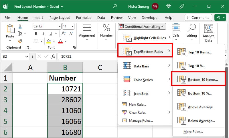
- Hover over Top/Bottom Rules and pick the Bottom 10 items.
- On the Bottom 10 Items window, decrease the number to 1. Choose a Shade you wish to highlight the value with and hit OK.
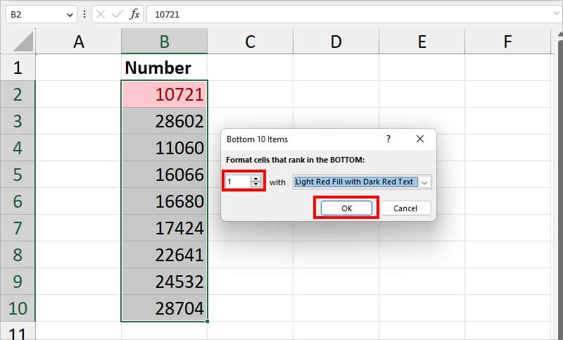
- Conditional Formatting will shade the Lowest Number.
Using MIN Function
Excel has an in-built MIN function that returns the smallest number from the data. I preferably use this function when I want to extract the minimum number separately.
Syntax: MIN(number1, [number2], [number3], ...)It only takes multiple numbers or cell references with numbers as a function argument. You could enter up to 255 numbers as an argument. However, remember, if there are no numbers in the cell references, you’ll get 0.
Example: Let’s assume you have the Student’s Name in Column A and English Test Scores in Column B. You want to find out the lowest score from the data. For this, you can use the MIN function as
=MIN(B2:B17)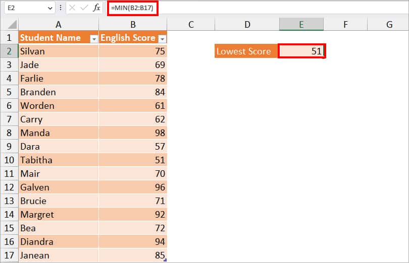
In the above formula, we simply passed down the arguments from cell B2 through B17. So, the MIN function looked for the smallest number within the specified cell ranges and returned 51 as a result.
Using SMALL Function
The MIN function returns the exact least number from the data. But, there can be situations when you would want to find the 2nd lowest or 3rd lowest number. During such cases, you could opt for the SMALL function.
The SMALL function returns the kth lowest value from the cell ranges.
Syntax: SMALL(array,k)This function takes up two arguments Array and K. Here, Array is the cell ranges to return the lowest value from. Similarly, K is the position of the lowest number.
Example: Let’s take the same example as above. But, here, let’s assume you need to find out the 3rd lowest scorer in English Test.
For this, we will use the formula as
=SMALL(B2:B17, 3)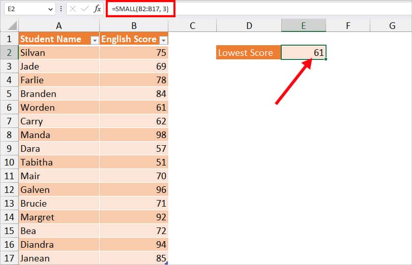
In the above formula, we have specified the SMALL function to return the 3rd smallest number from cells B2 through B17. So, we got 61 as output.
Setting a Minimum Rule in Conditional Formatting
In the first method, we used the pre-defined rule of Conditional Formatting. But, you can also set your own rule to locate and highlight the least number from your data. Here’s how you do it.
- On your sheet, select Cell ranges.
- From the Home tab, click on Conditional Formatting > New Rule.
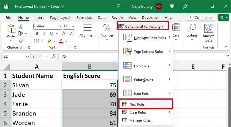
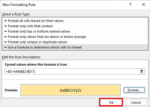
- On the New Formatting Rule window, pick Use a formula to determine which cells to format.
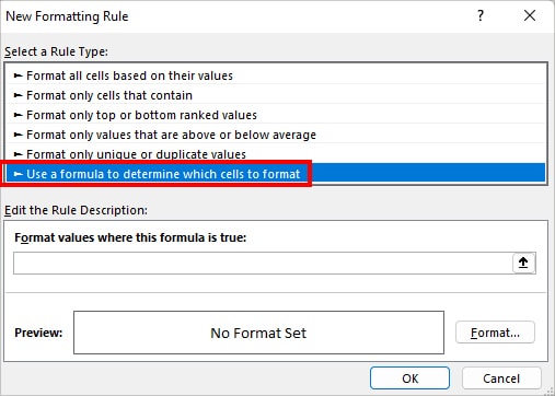
- Now, enter this formula
=B2=MIN(B$2:B$17).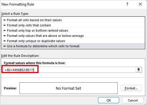
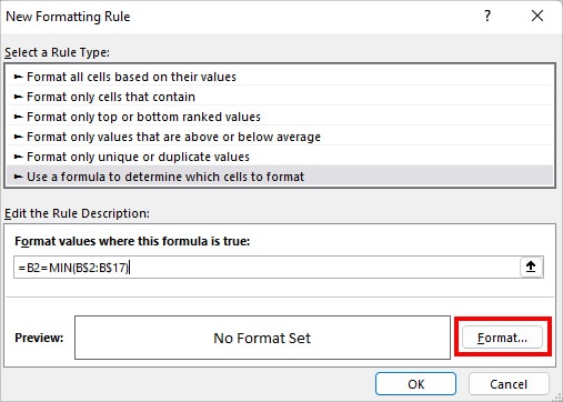
- Hit Format option.
- On Format Cells, navigate to the Fill Tab. Pick a Colour to highlight the value and click OK.
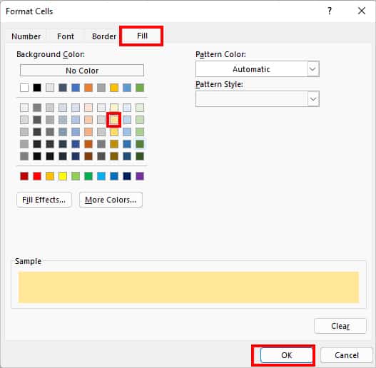
- Again, hit OK.
Using MINIFS Function
If you need to calculate the lowest number based on certain criteria, you could use the MINIFS function. The MINIFS function returns the lowest number just like the MIN function but with the specified condition.
Syntax: MINIFS(min_range, criteria_range1, criteria1, [criteria_range2, criteria2]...)Before we jump onto the example, let us first check out each argument that the MINIFS function takes.
- min_range: Array of Cell range to extract minimum value from.
- criteria_range1: Cell ranges to test the condition.
- criteria1: Criteria to test on Criteria range 1. It could be a Number, Text, Expression, etc.
- criteria_range2: Extra cell ranges to evaluate the criteria.
- criteria2: Additional criteria to evaluate.
Example: Let’s assume, you have the Science Test Scores of students in two groups. Here, you need to find the least score of each Group A and Group B.
For Group A, enter this formula.
=MINIFS(C2:C17, A2:A17, "A")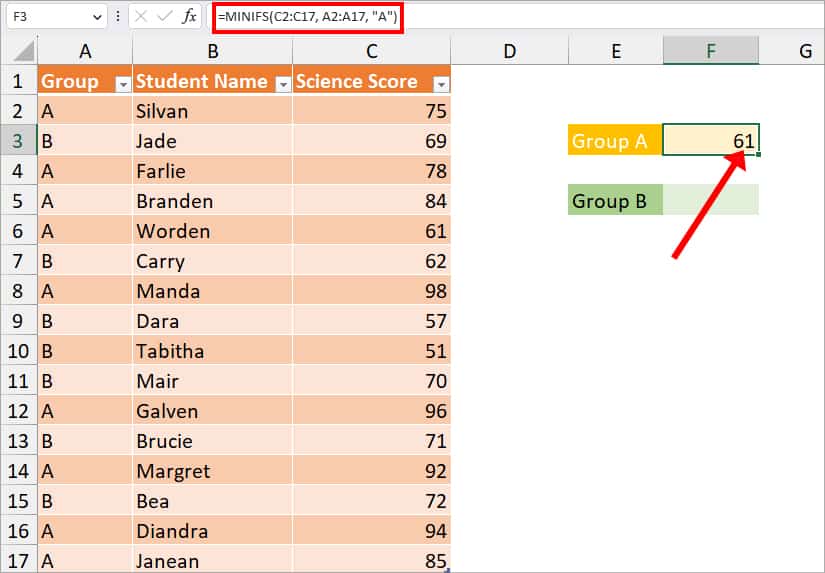
In the above formula, we passed down the cell range C2:C17 as criteria range 1. Similarly, A2:A17 is a criterion range2. Here, we specified “A” as the criteria for cells A2 through A17. So, the MINIFS function will return the lowest number of Group A which is 61.
Similarly, to find out the lowest scorer for Group B, your formula would be
=MINIFS(C2:C17, A2:A17, "B")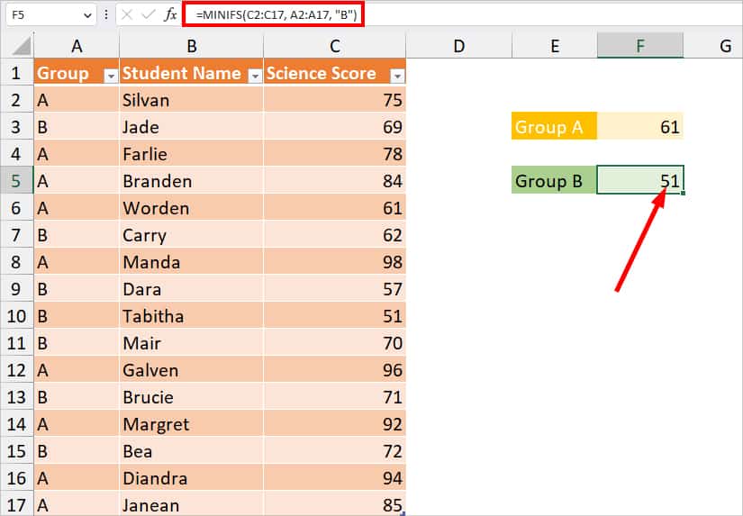
The formula looked for the smallest number in Group B from cell A2 to A17 and returned 51.
Using Nested Formula
So far we learned several methods to identify the smallest number from the data. But, sometimes, locating only the numeric value might not be enough. For Instance, if you have the Student’s test score, you would also want to find the student’s name with the least score.
While Conditional Formatting can help you with finding the related information, it is only best if both values are in the adjacent columns. So, here, we will nest MIN, MATCH, and INDEX, functions together.
| Function | Syntax | Description |
| MIN | MIN(number1, [number2], [number3], …) | Returns the least value from the selected range or numbers. |
| MATCH | MATCH(lookup_value, lookup_array, [match_type]) | Looks for the value in an array and returns its position. |
| INDEX | INDEX(array, row_num, [column_num]) | This function returns the item from a specified table or range. |
To determine the student name with the least score, use the given formula.
=INDEX(A2:A17, MATCH(MIN(B2:B17), B2:B17, 0))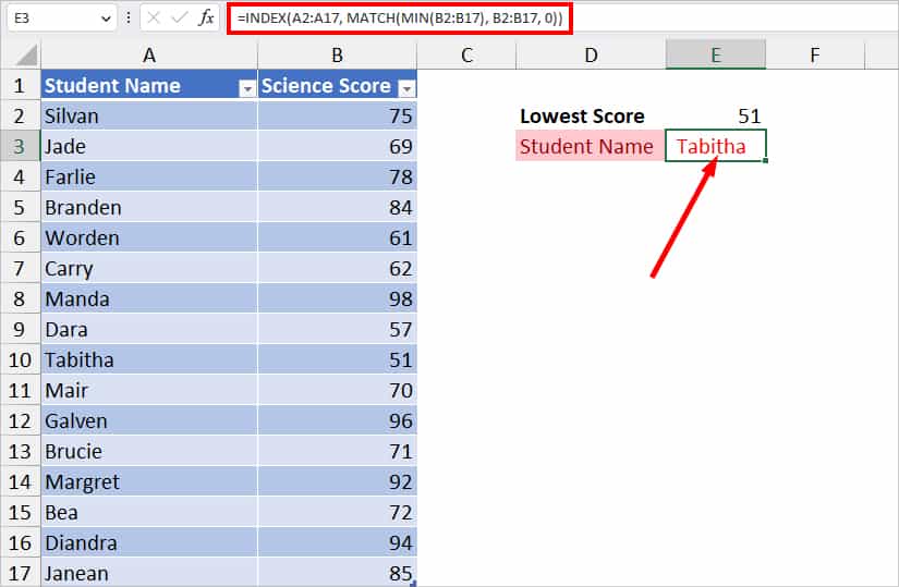
The formula returned Tabitha who scored the lowest in the Science Test. Now, let us understand how the formula returned the result.
- MIN(B2:B17): Firstly, the MIN function returns the lowest score from range B2 through B17 which is 51.
- MATCH(MIN(B2:B17), B2:B17, 0): This formula locates the relative position of 51 from B2 through the B17 array. Then, it returned 9th position.
- INDEX(A2:A17, MATCH(MIN(B2:B17), B2:B17, 0)): Finally, the INDEX function looks for the value of the 9th row from cell A2 through A17. Then, returns Tabitha as an outcome.