While analyzing statistical data, Outliers can put you at risk if you don’t find one soon and remove them. Why? Because these values can influence your findings and result in a wrong interpretation. In Excel, there are 5 ways to find Outliers. You could use the sort method, functions, or graphical representations.
What are Outliers?
Whether it’s in chart diagrams or data, Outliers are the unusual points that are noticeably far from the rest of the values.
For example, if you have 2, 3, -57, 9, and 100 in a dataset, -57 and 100 are the outliers. As you can see these values simply do not fit with the remaining values. But, of course, this is a very basic example.
In a real-life data analysis, Outliers are much more vague and have no distinct rule that defines them as one. It’s solely up to analysts to decide what makes the value an outlier in their respective datasets. This is why it’s up to you to choose the right method to identify such uncommon value.
Nonetheless, one thing you should absolutely note is that Outliers negatively impact your statistical analysis. These points tend to distort the result and lead to misinterpretation of the findings. So, what do you do after detecting an Outlier? Remove them!
Having said that, it’s a very rare case, but the Outliers can sometimes have significant information. Before you delete them, I suggest you check and analyze how those points appeared first.
Sort your Data
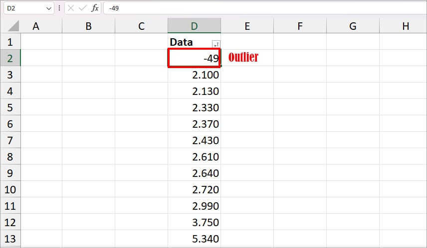
If you have a small record, you can sort your data in ascending as well as descending order to detect the outliers. In this method, we will re-arrange the values and look for the existing outliers by ourselves. While it’s simple to use, it can be tedious for large datasets.
Firstly, let’s arrange the numbers in ascending order. Click on the Cell and enter Ctrl + Shift + L shortcut key for Filter. Select the Filter icon and choose Sort Smallest to Largest.
Now, look for a distinct value that is unusually small in a couple of first-cell ranges. If you find one, it’s an outlier.
Again, let’s reorder the values in descending order. Click on Filter tool > Sort Largest to Smallest.
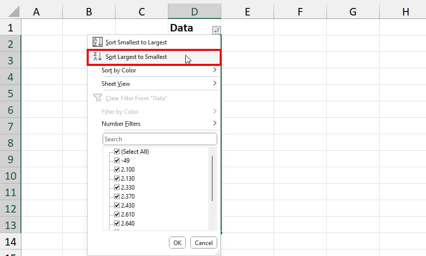
Now, look at the topmost value and a few cell ranges below it. Do you notice an extraordinarily large number than others? If so, it’s an Outlier.

Using LARGE and SMALL Functions
For a large number of columns, it isn’t possible to sort the columns in order one by one and look for outliers. To avoid this hassle, you can use Excel’s LARGE and SMALL functions. Basically, these functions return the nth highest and nth lowest values from the cell ranges.
Example 1: LARGE Function
Suppose, if I wish to check the 3rd largest number, I will enter the formula as
=LARGE(B3:B13, 3)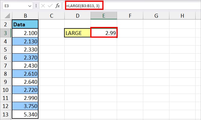
In the formula, cell ranges from B3 through B13 is our array to return the number from. Here, we have specified 3 as the position to return. Hence, we got 2.99.
Example 2: SMALL Function
We will take the same example again. But, use the SMALL function to get the 4th lowest value. For this, I used this formula
=SMALL(B2:B13, 4)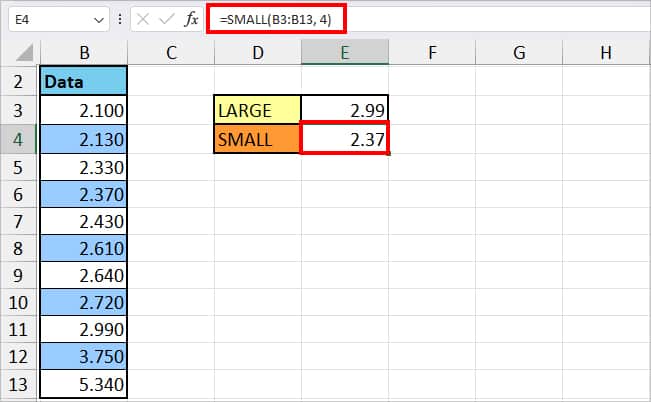
The SMALL function resulted in the 4th smallest number from B3:B13 which is 2.37.
Using InterQuartile Range
Next, in Statistics, the InterQuartile Range is also used to identify the Outliers from the Data. It is especially helpful for extremely big datasets. Here, we will first calculate the InterQuartile Range Value of the data and check for the Outliers. The best part is there is a QUARTILE.INC function to find out the value of Q1 and Q3.
To detect the Outliers using the InterQuartile Range, there are a few things you would have to calculate like First Quartile (Q1), Third Quartile (Q3), InterQuartile Range, Upper Bound, and Lower Bound.
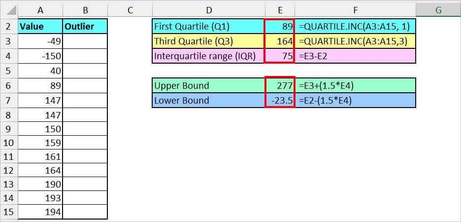
Example: Suppose, I have a list of Data in the cell range A3:A15. Before you start, I recommend you sort the numbers in ascending order.
| Calculate | Formula | Output | Description |
| First Quartile (Q1) | =QUARTILE.INC(A3:A15, 1) | 89 | In the formula, we have specified the A3:A15 array and 1 to find out the value of Q1. |
| Third Quartile (Q3) | =QUARTILE.INC(A3:A15, 3) | 164 | Using the same QUARTILE.INC function, we have passed down the A3:A15 array and 3 to return Q3 this time. |
| InterQuartile Range Formula: (Q3 -Q1) | =E3-E2 | 75 | For, the InterQuartile range, we’re simply subtracting the value of Q3 in cell (E3) by Q1 (E2). |
| Upper Bound Formula: Q3 + (1.5 *IQR) | =E3 + (1.5*E4) | 277 | In this formula, we have passed down the UPPER bound formula to calculate the value. Here, E3 is the value of Q3 and cell E4 is IQR. |
| Lower Bound Formula: Q1 – (1.5 * IQR) | =E2-(1.5*E4) | -23.5 | We’ve entered the Lower Bound Formula where cell E2 is Q1, and E4 is IQR. |
Now, that we have all the required values, we will use the IF and OR functions nested to test multiple criteria and return TRUE or FALSE Boolean. Basically, if the cell has a TRUE result, it means that the number is an outlier.
We entered the formula as in the box and copied it down for the other ranges.
=IF(OR(A3<$E$7, A3 >$E$6), TRUE, FALSE)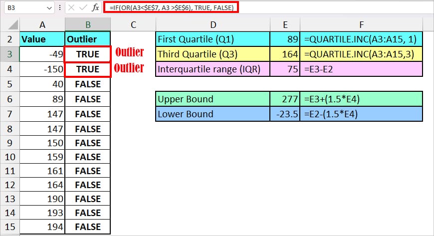
The formula resulted in TRUE or FALSE. Here, the value of cells A3 and A4 got TRUE. So, these are the Outliers.
Let’s dive into the formula in more detail.
- OR(A3<$E$7, A3 >$E$6): First of all, the OR function tests two logic which is either the value of A3 is smaller than the Lower Bound. Or, the Value of A3 is greater than the Upper Bound. It returns a Boolean value for the test. In this instance, we got TRUE.
- IF(OR(A3<$E$7, A3 >$E$6), TRUE, FALSE): Now, the IF function takes OR(A3<$E$7, A3 >$E$6) as a logical test. Then, when the value is correct, it results in TRUE and if it’s incorrect, you’ll get FALSE. Since the OR function returned TRUE, we got TRUE as a final result.
Using Scatter Diagram
When you plot a Scatter Diagram with Outliers, you’ll see that the outlier variable lies far from the graph’s trendline. So, it is one way to find out the value that does not fit in the plot. This method is especially useful when you need to conduct a regression analysis.
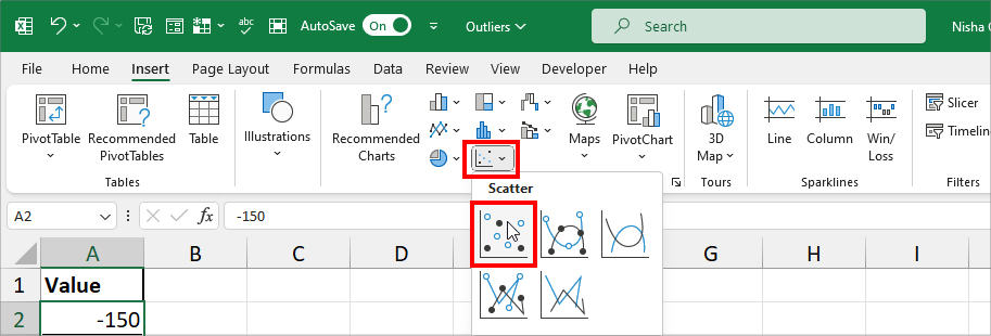
- Select your data and go to the Insert Tab.
- From the Charts section, click on Scatter and choose Scatter chart.
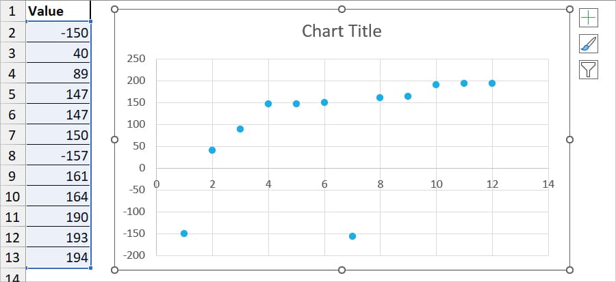
- You’ll have a Scatter Chart.
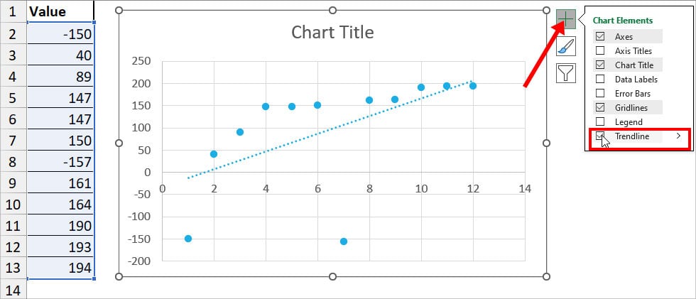
- To add a Regression Line, select the + icon in the chart area. Then, tick the box for Trendline.
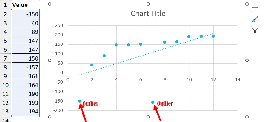
- Now, observe the graph and see the data series that’s way too far from the trendline. In our case, -150 and -157 are Outliers.
Using Box Plots
Box Plots visually represent the data of Q1, Q3, and IQ in the chart. If you use Excel 2016 and later versions, you don’t even have to calculate such values to construct a box plot. But, for older versions, you need to find out the values prior to creating the chart.
After you insert a box plot, the graph shows the Outlier point by default in the Chart Area. While you can add a Box Plot for a single column, this method is especially great for users who have two or more columns to detect the Outlier.
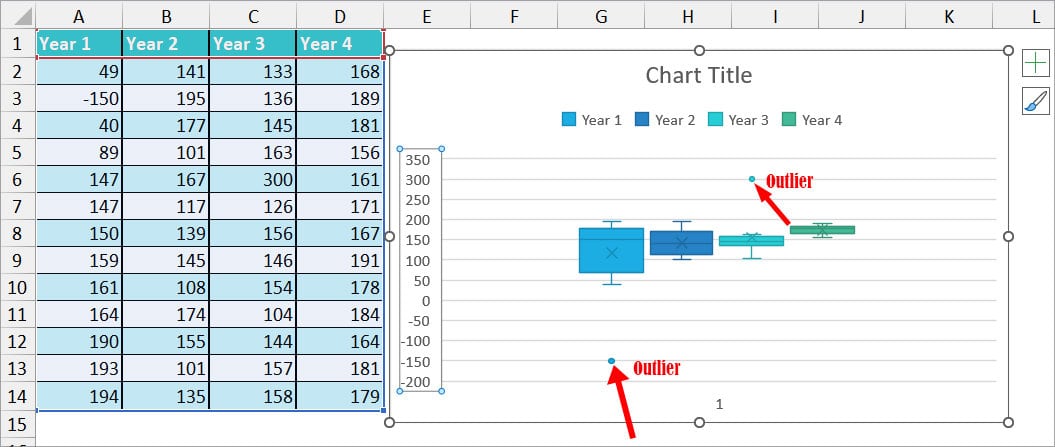
Example: Here, I have the values for Four Years – Year 1, Year 2, Year 3, and Year 4. Let’s identify the Outliers in all these Years just by using one Box Plot.
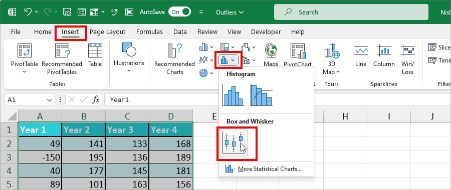
- On your sheet, select all data.
- On the Insert Tab, hover over the Charts group. Click on Histogram and pick Box and Whisker.
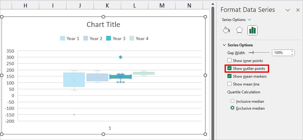
- If there’s an Outlier, you’ll see a Point either above or below the box plot. In our case, Year 1 and Year 3 have an Outlier.
In case, your chart does not show an Outlier mark, right-click on any one Box plot and choose Format Data Series. Below the Series Options, tick the option for Show outlier points and close the sidebar.