How to Draw a Circle in Excel

While a circle may seem just a basic shape, it can serve many purposes in Excel. For Instance, you could draw circles to highlight cell values in your sheet. Or maybe use circles to create decision trees, progress bars, circle graphs, and many more. Depending on your need, you could either draw a shape or use the pre-built circle designs. 

Draw Shapes

Firstly, you could draw a circle from the Shapes icon in Excel. This method is for users who just want a basic circle shape. It can be useful to highlight the cell values with a circle, create chance nodes for the decision tree, build flowchart diagrams, etc. 

Inserting shapes in Excel is pretty easy. Here, you just need to select a circle shape and draw the shape just like in the Paint program.

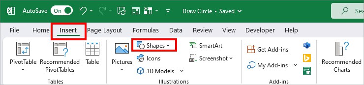
1. On your worksheet, head to Insert Tab.
2. From the Illustrations section, click on Shapes.
   
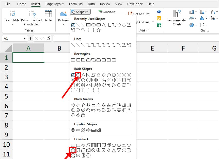
3. Under Basic Shapes, click on Oval shape. (For Flowchart diagrams, click on Flowchart: Connector shape under the Flowchart category)
   
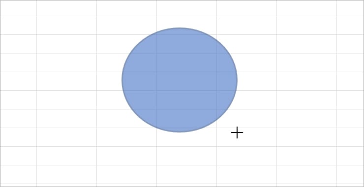
4. Then, using the Plus cursor, draw a Circular shape on your sheet.
   
5. To edit the shape, select the Circle and go to Shape Format.
   
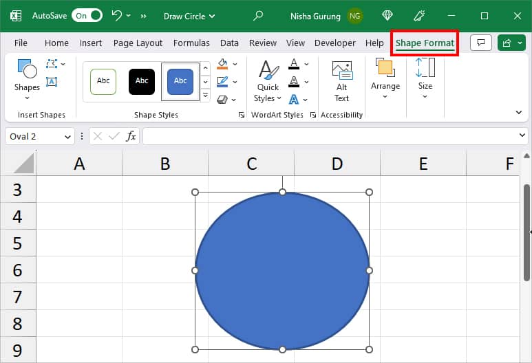
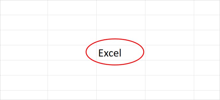
6. Change Shape Styles, Size, Shape Oultine, Shape Fill, and many more. Here, to highlight the cell value, we set the Circle to No Fill in Shape Fill. Then, picked a Red color for the Shape Outline.
   

Insert SmartArt

SmartArt shapes are mostly used to illustrate the relationship and process in a figure. Here, you can find several in-built designs of circles grouped together. Also, when you select a design, a short description of the figure appears at the bottom. Choose and insert one of the designs. 

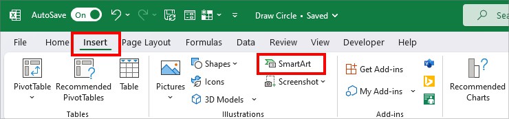
1. On your Excel worksheet, go to Insert Tab.
2. From the Illustrations group, click on SmartArt.
   
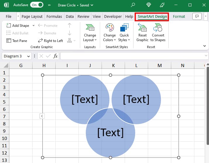
3. On Choose a SmartArt Graphic window, browse through each category on the left and pick a Circle Design. Here, we selected the Interconnected Rings design from the Relationship category.
   
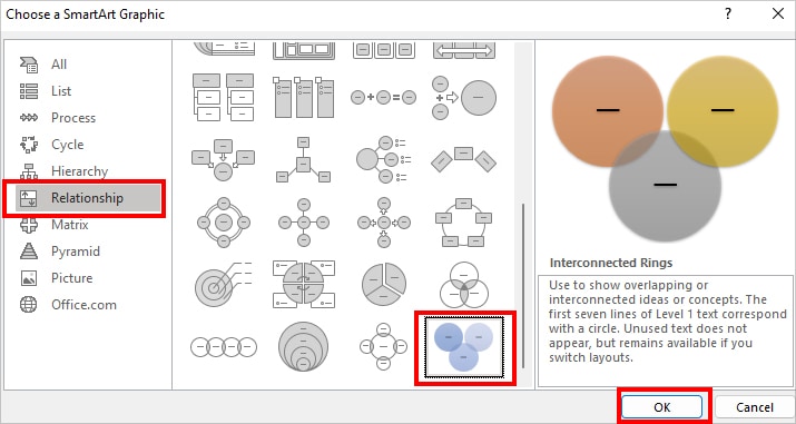
4. Click OK to insert the circle.
5. To modify the design, select the Shape and head to the SmartArt Design tab.
    
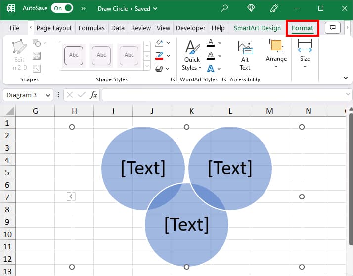
6. To format Shape, navigate to Format Tab while the circle is still selected.
    

Insert Doughnut/Pie Chart

For more advanced circle shapes, you can insert Excel charts as required. Excel has Doughnut, 2-D and 3-D Pie Charts. As an example, here, we will add a doughnut chart to create a progress bar.

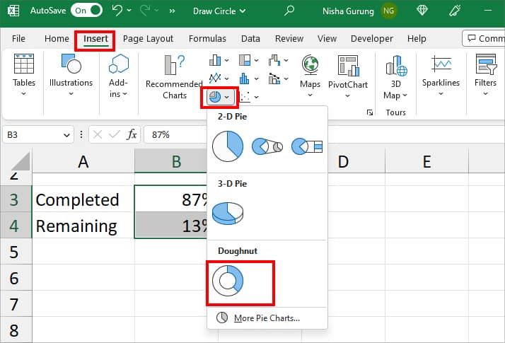
1. Firstly, select the Completed and Remaining data on your sheet.
2. Navigate to Insert Tab. From Charts section, select Pie-Chart and click on Doughnut Chart.
   
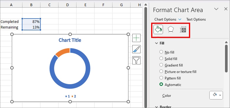
3. Click on the Doughnut Chart twice to bring up the Format Chart Area menu. Go to each Fill & Line, Effects, and Size & Properties menu to edit the chart.
   

Insert Scatter Chart

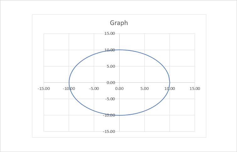
Sometimes, you may have to create a circle graph in Excel out of the Angle and Radius. We will be using a Scatter Chart to represent the value of XY coordinates. Here, your data must have a total 360-degree angle in order to form a circle in the Scatter diagram. 

We will first find the values of X and Y. Then, plot a scatter chart. In case you already have all the required data, you can directly begin with Step 2.

Step 1: Find the Values of X and Y

There’s a formula to input the values of angles instead of entering them one by one. For this, start with a 0 value in a new cell. Then, enter 15 in the next cell. Now, in the third cell, use the formula in the box. Extend the Flash-fill handle until you get the 360 value. 

=A8 + $A$8

Now, you have all angle in Column A. Let’s suppose, we have 10 as Radius. To find the value of X, we will use the COS and RADIANS functions nested together. Enter the formula as

=D7*COS(RADIANS(A7))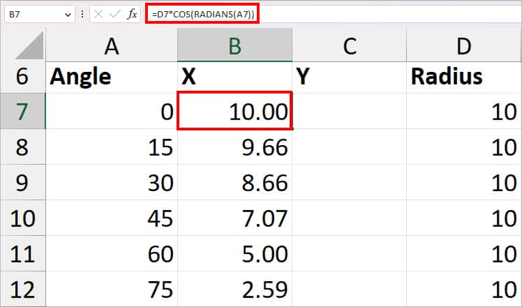

Here, the RADIANS(A7) formula first returns a 0-degree angle as radians. Then, the COS function returns the cosine of an angle which is 1. Finally, the result is multiplied by the value of Radius in cell D7 and returns 10 as an output. Use Flash-fill handle for other cells too.

Now, to find out the value of Y, we will use the SIN and RANDIANS functions. Enter the formula mentioned in the box below.

=D7*(SIN(RADIANS(A7)))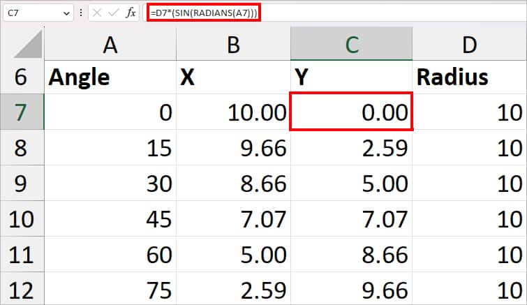

Firstly, the RADIANS function returns the degree of A7 cells as radians. Then, the SIN function returns the angle to Sine and returns 0 according to our value. Finally, when the radius multiplies the 0 value, you will get 0. Drag the Flash-Fill handle to fill in the rest of the value of Y.

Step 2: Plot Scatter Chart

1. On your sheet, select the X and Y values. 
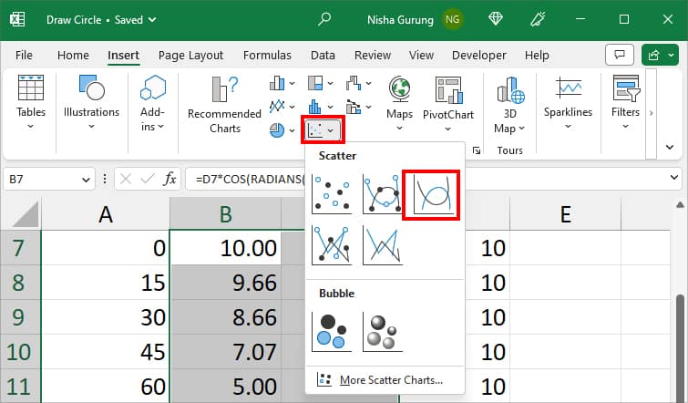
2. Head to Insert Tab and hover over the Chart group.
   
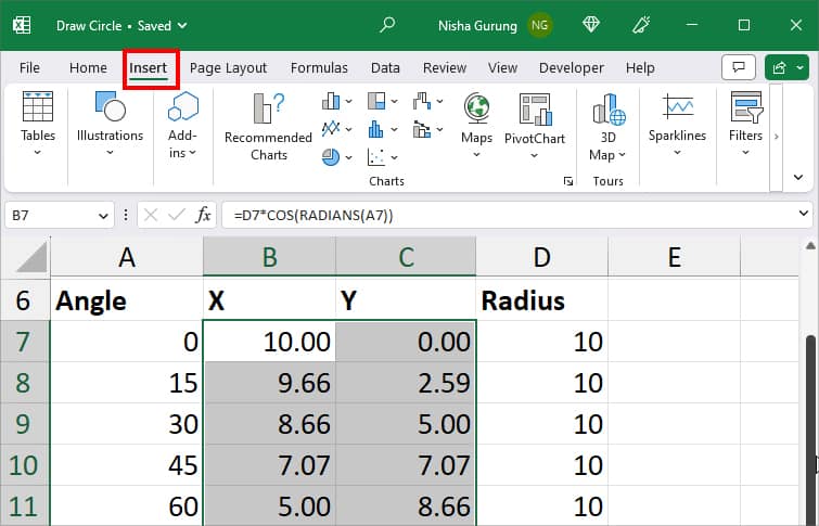
3. Select Scatter > Scatter with Smooth Lines.
   
4. You’ll have a circular scatter chart on your sheet.