Excel has two functions, FACT and FACTDOUBLE to calculate two different types of factorials. Both, FACT and FACTDOUBLE fall under the Math & Trig functions and are used mostly to generate permutations and combinations.
The FACT function computes the standard factorial (n!) of a number, while the FACTDOUBLE function calculates the double factorial of a number. While using these functions is relatively simple, you may sometimes encounter the #NUM! Excel error.
In this article, we will be covering everything about the application of these functions, including how you can avoid the #NUM! error.
What are Factorials and Double Factorials?
Most of us must be familiar with factorials than double factorials. Factorials are the product of all whole numbers from 1 to the set value.
Mathematically, a factorial is denoted by the exclamation mark (!). For example, 5! = 1x2x3x4x5 which results in 120.
Double Factorials on the other hand are the product of a number from its lowest parity to the set number. In simple terms, the double factorial of an odd number begins with 1 while the double factorial of an even number begins with 2. A double factorial is represented by double exclamation marks (!!).
For example, 9!! = 1x3x5x9 which is 945. Similarly, 8!! = 2x4x6x8 which is 384.
Calculating Factorial in Excel
A single factorial, or an n!, is calculated using the FACT function in Excel. The FACT function requires only one argument, which is the number you wish to calculate the factorial of. The FACT function is written in the following format when constructing a formula:
=FACT(number)Here’s a table showing what argument returns what value using the FACT function in Excel.
| Number | Formula | Result | Description |
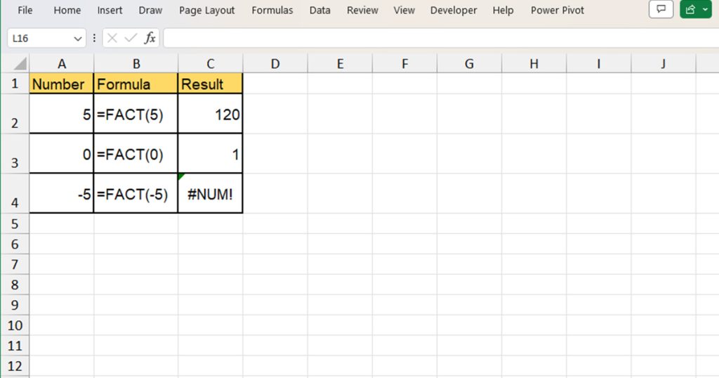
| 5 | =FACT(5) | 120 | The factorial of 5 is 120. |
| 0 | =FACT(0) | 1 | The factorial of 0 is 1. |
| -5 | =FACT(-5) | #NUM! | You can only calculate the factorials of numbers greater than 0. |
Calculating Double Factorial in Excel
Excel also has a dedicated function, FACTDOUBLE to calculate the double factorial of a number. Similar to the FACT function, the FACTDOUBLE function also requires only one argument, which is the number you wish to generate the double factorial value for.
The FACTDOUBLE function is constructed in the following way when writing a formula:
=FACTDOUBLE(number)Check out this table to see what argument returns what value when using the FACTDOUBLE function in Excel.
| Number | Formula | Result | Description |
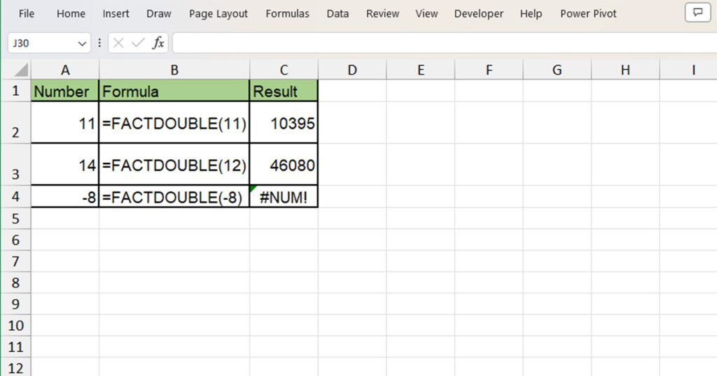
| 11 | =FACTDOUBLE(11) | 10395 | The product of 1x3x5x6x7x9x11 is equal to 10395. |
| 14 | =FACTDOUBLE(14) | 645120 | When you multiply 2x4x6x8x10x12x14, you will get 645120. |
| -8 | =FACTDOUBLE(-8) | #NUM! | You cannot calculate the double factorial of a negative number. |
What is a #NUM! Error in Excel?
In both of our examples using the FACT and FACTDOUBLE functions, you may have noticed that passing a negative number as an argument results in the #NUM! Error. Most of us already know that it is not possible to calculate the factorial or the double factorial of a negative number. However, you might be wondering what exactly is the #NUM! error code in Excel.
Well, the #NUM! error code is Excel’s way of alerting you that the numeric value you entered in your argument does not result in a valid result. As a negative number is an invalid argument, Excel triggered the #NUM! error.
Use IFERROR to Avoid #NUM!
If you’re not a fan of seeing error codes in Excel, you can nest your functions inside the IFERROR function. Especially if you’re a teacher, you can nest every function inside the IFERROR function so if someone enters a number that results in an error, you can display a custom message instead of the error.
For example, =IFERROR(FACTDOUBLE(-8), "Use a Positive Number") returns “Use a Positive Number” instead of the #NUM! Error. You can also use the IFERROR function while creating templates to fill in numbers later.