When importing data on Google Sheets, you may encounter junk data on every other row. To clear such data, simply filter the rows to display only alternate rows, make your selection, and then delete them.
Also, Google Sheets offers advanced data filtering that allows you to filter specific data using formulas.
For example, you can use the ISODD function to filter odd-numbered rows or the ISEVEN function to filter even-numbered rows.
If you’re looking to delete every nth number of rows, filter the rows using the MOD function.
Remove Every Odd Row
| Function Used | Data Type | Syntax |
| ISODD | BOOLEAN | =ISODD(value) |
| ROW | LOOKUP AND REFERENCE | =ROW(cell_reference) |
The ISODD function in Google Sheets returns TRUE or FALSE based on whether the referenced value is odd or not.
We can filter criteria using the ISODD and ROW functions. Using this formula, Google Sheets will filter out all even rows. Then, we can delete the odd-numbered rows from our grid.
- Select your column header.
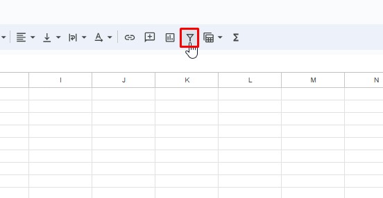
- From the menu bar, click on the filter option.
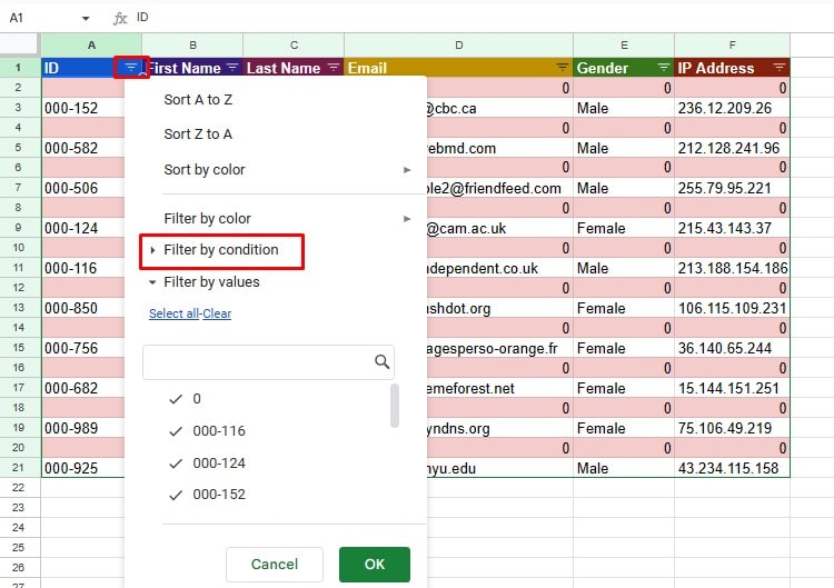
- Back on your sheet, select the filter button on your column header.
- Expand Filter by condition.
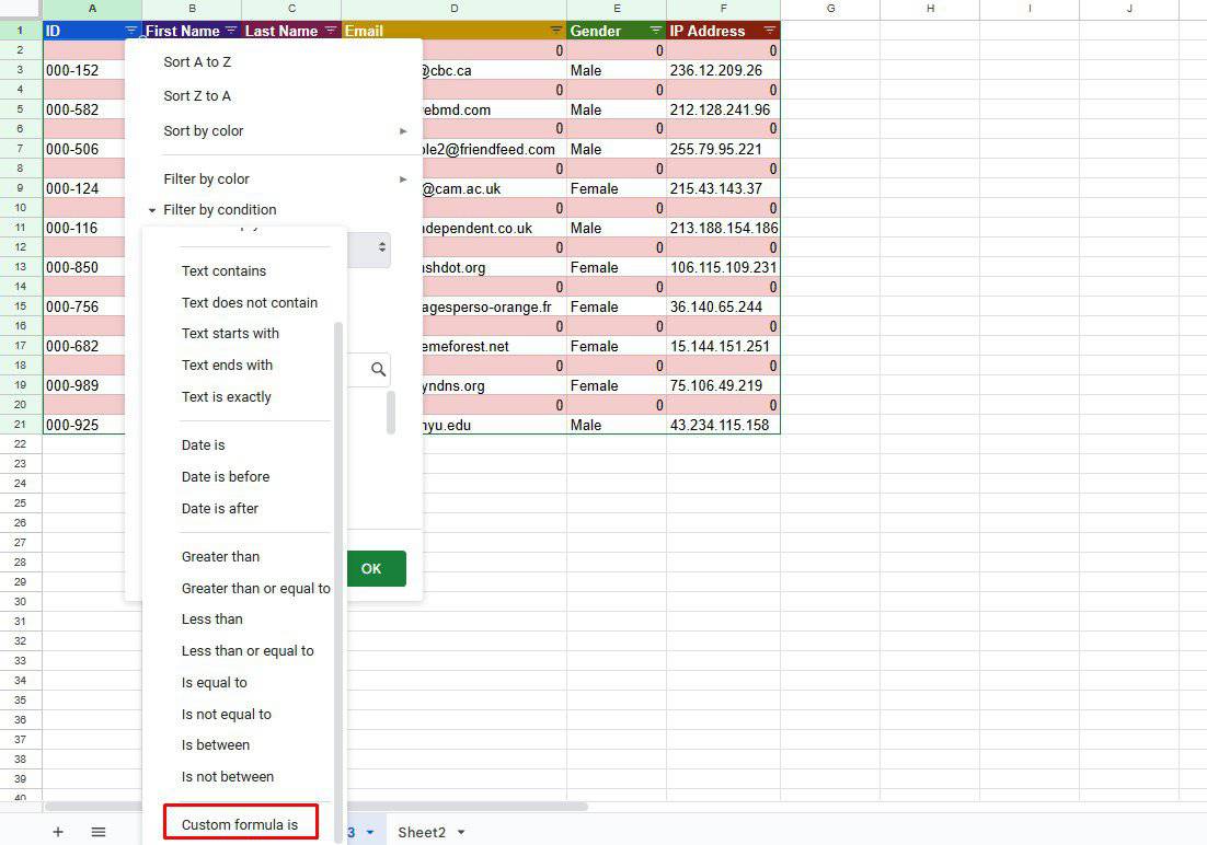
- Select the fly-out menu and choose Custom Formula is
- In the value or formula section, enter the following formula:
=ISODD(ROW(A1:A21))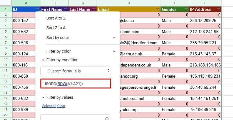
- Click OK.
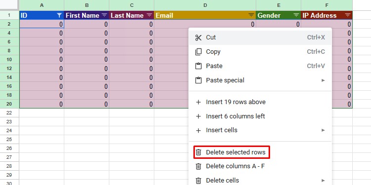
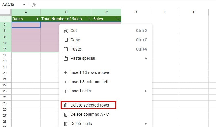
- Select your rows. Then, right-click on them and choose Delete selected rows.
- Right-click on the column header.
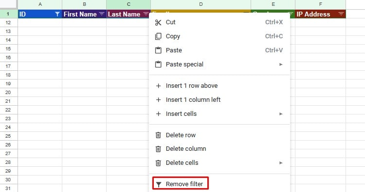
- Choose Remove Filter.
Remove Every Even Row
| Function Used | Data Type | Syntax |
| ISEVEN | BOOLEAN | =ISEVEN(value) |
| ROW | LOOKUP AND REFERENCE | =ROW(cell_reference) |
The ISEVEN function is the exact opposite of the ISODD function in Google Sheets. ISEVEN returns TRUE or FALSE based on whether the referenced number is an even value.
If you want to filter out the odd numbers to delete the even-numbered rows, use the ISEVEN function instead. We will again insert a filter and then delete the even-numbered rows.
- Click on the column header.
- Select the Filter option from the menubar.
- Click on the filter option from the column header.
- Expand Filter by condition.
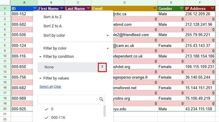
- Click on the fly-out and select Custom Formula is.
- Enter the following formula in the value or formula section:
=ISEVEN(ROW(A1:A20))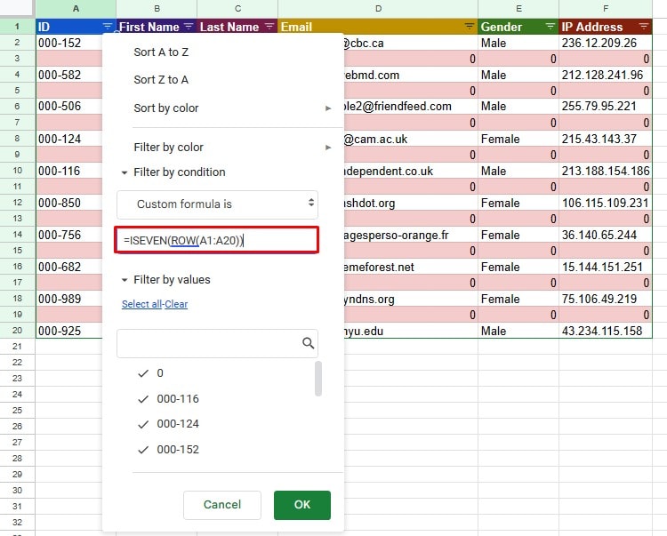
- Select OK.
- Select the range and right-click on it.
- Choose Delete selected rows.
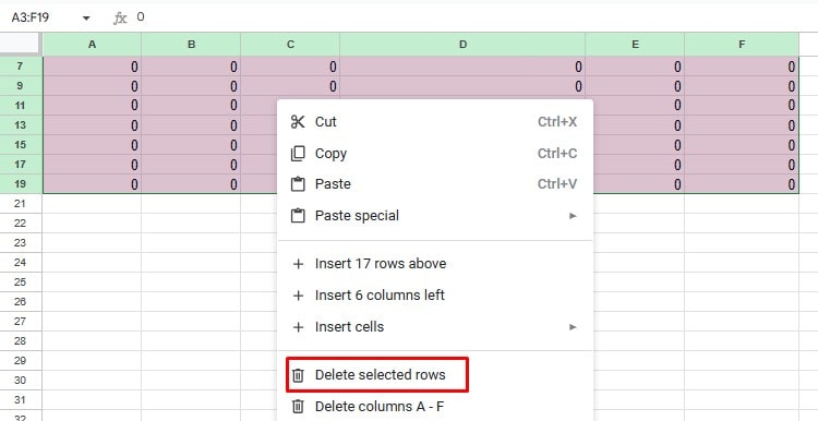
- Right-click on the column header and select Remove Filter.
Remove Every Nth Row
| Function Used | Data Type | Syntax |
| MOD | INTEGER | =MOD(dividend, divisor) |
| ROW | LOOKUP AND REFERENCE | =ROW(cell_reference) |
Say, you want to set a rule to delete rows after every 3rd row. In such cases, you can filter the column using a formula with the MOD function.
The MOD function calculates the remainder value using a dividend and a divisor.
As an example, let’s delete every two rows in Google Sheets. To create our formula, we’ll first have to analyze the data table.
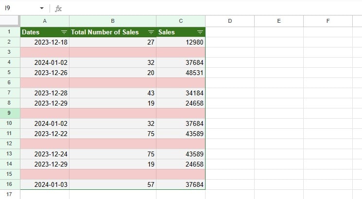
Here, every target row is divisible by the number three. So, we can create a condition to only show rows where MOD returns 0 when ROW is the dividend.
- Select range A1:E16.
- From the menu bar, click Data > Insert filter.
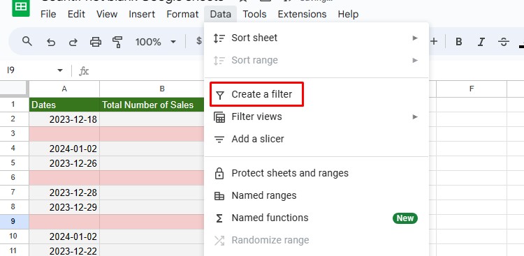
- Click on the filter option on the column header.
- Expand Filter by condition.
- Select the fly-out > Custom Formula is.
- In the Value or Formula section, enter the following formula:
=MOD(ROW(A2:A16),3)=0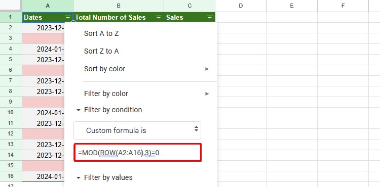
- Click OK.
- Select the entire range and right-click on it.
- Click Delete selected cells.
- Go to Data > Remove filter.
