Everyone has their own way of recording information in an Excel sheet. If you’ve imported a spreadsheet, there are possible chances some values are entered in separate columns. For Example, the Area Codes and Phone Numbers could be in two different columns.
When the data are placed in each individual column, some of them can be worthless on their own. You wouldn’t want the username and domain name of an email address separately, right?
In that case, it is best to combine two columns together. Here, when we say combine, we won’t be merging cells. But instead, we will join the values of different columns into one. We have compiled five methods to do so in this article. Keep reading!
Using Flash Fill
Excel’s Flash fills are one of the most interesting features used to separate, join, or format values in a certain way. When Flash fills recognizes a particular pattern in the data, it’ll automatically refill the remaining value. So, what better way to combine two columns in Excel than using Flash Fill?
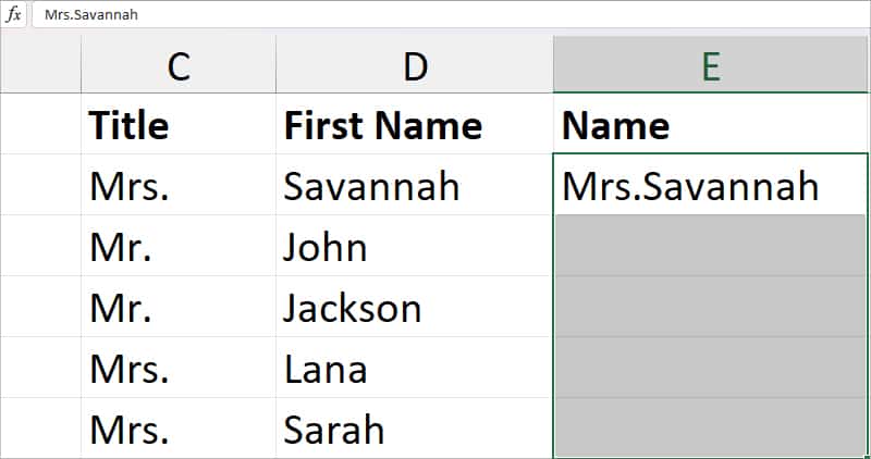
Example: Let’s suppose you need to combine the Title in Column C with the Name in Column D.
In a new column, firstly, type in the joined text which is Mrs.Savannah and press enter. Then, simply enter Ctrl + E keyboard shortcut to auto-fill the remaining cells.
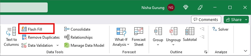
Alternatively, you can also find the Flash-fill in the Excel Ribbon.
- Select the value you just entered and the remaining cells.
- Head to the Data Tab.

- From the Data Tools group, click on Flash Fill.
Using Ampersand Operator
In Excel, the Ampersand character (&) combines two items from different cells. So, let us use this symbol to join two columns together.
Here, the rule is pretty simple. You just need to enter the & character between two cell references. To add a space, you can insert a space enclosed inside the double quotation mark (“ ”) in between the cell references.
Check out these examples to learn how to merge columns using this character.
Example 1: Join Columns Without Space
Let’s say you need to join the usernames of Column B and the domain names of Column C to create an address. For this type of data, you don’t need any space between the merged texts. So, your formula would be
=B4&C4
The Ampersand operator combined the value of cells B4 and C4. Then, returned [email protected]. Extend the Flash-fill handle to apply the same formula for other data too.
Example 2: Join Columns with Space
If you wish to separate two joined texts with a space, we will add a (“ ”) space in between the cell references in the formula. Suppose, you need to combine the pieces of address from Columns A, B, and C.
For this enter the formula as
=A1&" "&B1& " "&C1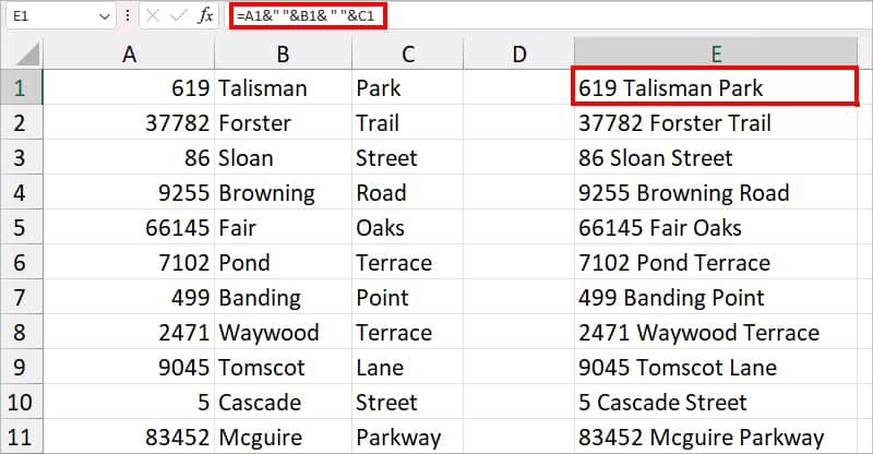
The Ampersand operator combines the value of each Column A1, B1, and C1. Since we passed down space in between each cell reference, it returned 619 Talisman Park as a result.
Example 3: Join Columns with Delimiter
Some values require a delimiter while combining them. For Example, you have the Phone code and Phone Number in a different column. To join these columns together, you might want to add a dash delimiter.
Now, for this, we will pass down a dash delimiter in the formula just like how we added space above.
=A4&"-"&B4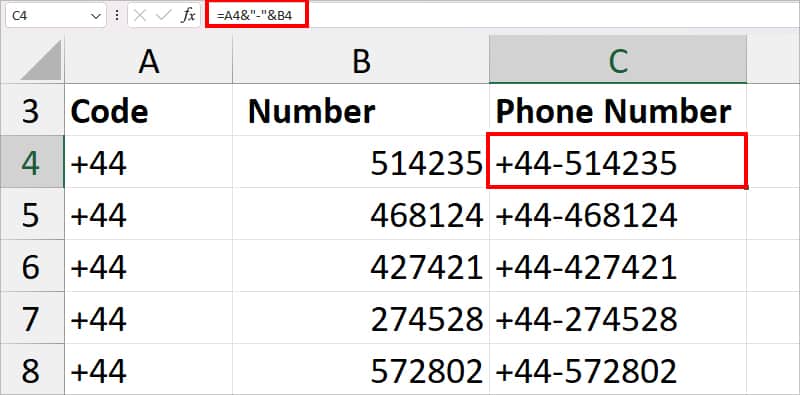
The Ampersand character joined cells A4 and B4 with a dash in between. As a result, it returned +44-514235.
Using CONCAT Function
In most cases, users opt for the Ampersand operator to join columns without using any function. But, it still is a tedious process and prone to errors as you need to keep adding the operator after each cell reference. To cut this, Excel has a default CONCAT function with the same functionality as the Ampersand character.
I personally use the CONCAT function as I find it easier to enter the cell references in the Formula. Also, note that this function is the replacement for CONCATENATE function. Since Excel marked CONCATENATE as a compatibility function, we highly recommend you use the CONCAT function.
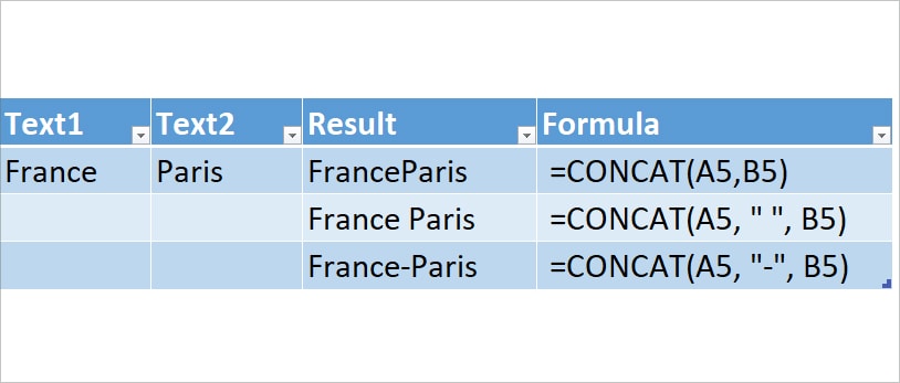
Syntax: CONCAT(text1, text2, text3,.....) The arguments of the CONCAT function are text1, text2, text3, etc. Excel allows you to enter 255 arguments at a maximum. Similar to the Ampersand operator, you can use the CONCAT function to combine columns without space, with space, and with a delimiter. Let’s check all of these examples from the table.
| Example | Text 1 | Text 2 | Formula | Description |
| Without Space | France | Paris | =CONCAT(A5,B5) | The formula concats the values of cells A5 (France) and B5 (Paris). Then, returns FranceParis as an output. |
| With Space | France | Paris | =CONCAT(A5, “ ”, B5) | In this formula, we’ve entered a space inside the quotation mark. So, now, the formula returns the space between two values. As a result, we got France Paris. |
| With Delimiter | France | Paris | =CONCAT(A5, “ – ”, B5) | Here we passed down a dash delimiter “-” in the formula. So, now, it returned France-Paris. |
Using TEXTJOIN Function
You must have noticed with the Ampersand character and CONCAT function, you need to enter a delimiter each time in the formula. Now, this can be monotonous work if you have more than two columns to combine.
Luckily, Excel’s TEXTJOIN function is built just to return the joined values with the specified delimiter. So, you could opt for the TEXTJOIN function to quickly combine columns that involve a delimiter.
Syntax: TEXTJOIN(delimiter, ignore_empty, text1, text2, text3,.....)The function argument of TEXTJOIN are:
- delimiter: Character to insert in between the texts. It should be enclosed in double quotation marks. [required]
- ignore_empty: specify whether to ignore or accept the blank cells.
- text1: first cell to join
- text2: second cell reference to join
Example: Suppose you have a Country code, Area code, Prefix, and Line Number in four different columns. Let’s say you need to merge all these numbers together with a dash delimiter to form a number. For this, enter the formula given in the box.
=TEXTJOIN("-", TRUE, A2:D2)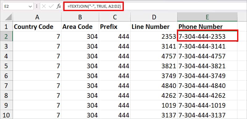
In the formula, we passed down a “-” delimiter to combine values of columns from cells A2 through D2. So, the formula returned 7-304-444-2353. You can extend the fill handle for the other remaining cells.
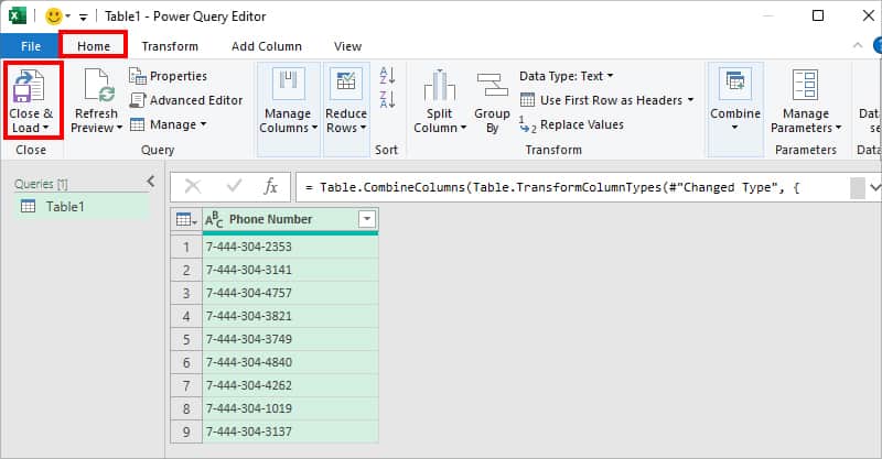
Using Power Query
If you do not want to use formulas to merge columns, this method is best for you. Here, we will use Excel’s Power Query Editor tool to combine columns and load them.
- Select an entire data.
- From the Data Tab, click From Table/Range menu.
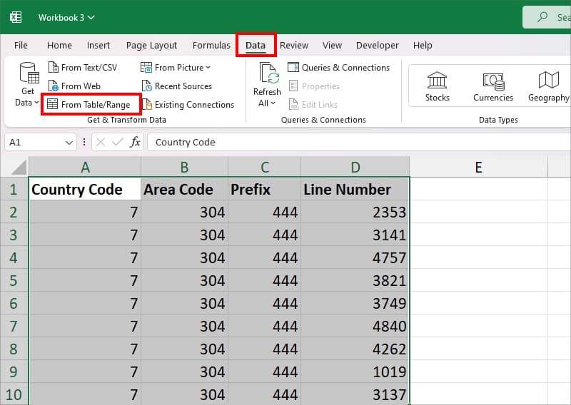
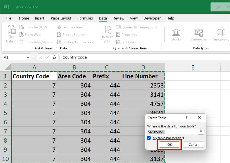
- If prompted, click OK.
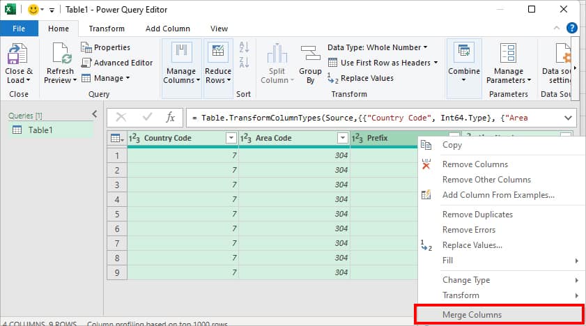
- On Power Query Editor window, select the Columns to combine by holding down the Ctrl key.
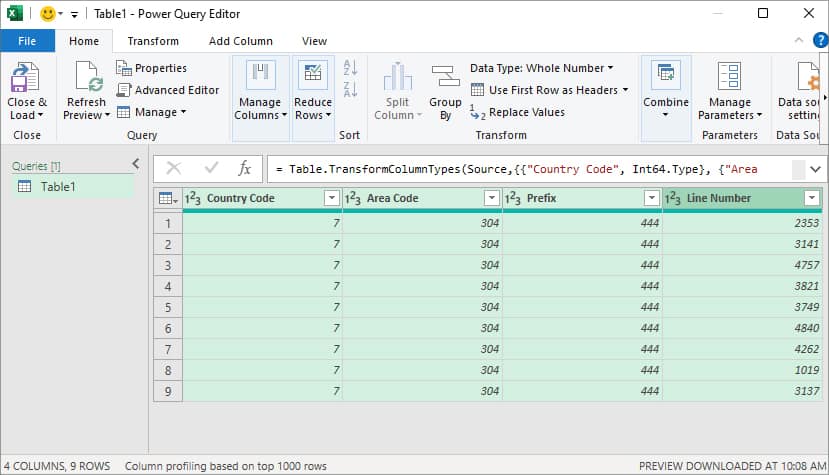
- Right-click on the Column Header. Then, pick Merge Columns.
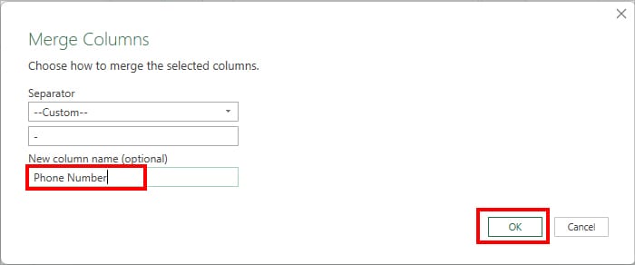
- On Merge Columns window, set a Separator. Here, we chose Custom and entered a dash (–).

- Below New column name, enter a Name as you wish. When done, hit OK.
- On Home Tab, click Close and Load.