How to Capitalize All Letters in Excel

Imagine working on a spreadsheet for hours only to later realize that certain data needed to be in uppercase.

This happens more than you think. This could be why Excel has not just one, but three different ways to capitalize all letters in Excel.

You can use the UPPER function, Power Query to transform your text into uppercase, or even use Excel’s smart AI to autofill capitalized data.

Use UPPER Function

UPPER is a dedicated text function in Excel, used to capitalize the text you pass as a reference. The UPPER function has a pretty basic syntax. This is how you can write UPPER when constructing a formula:

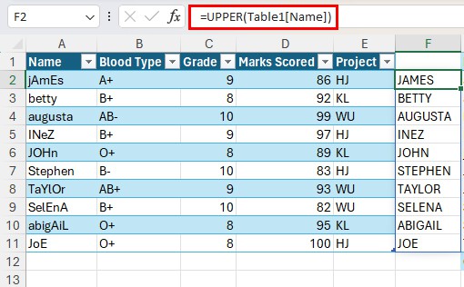
=UPPER(text)

In range A2:A11, I have ten names in mixed and lower cases. Let’s use the UPPER function to capitalize all letters from this range.

=UPPER(A2:A11)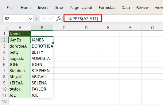

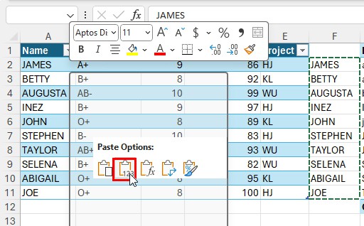
Remember, if you want to replace the data, paste the formula results as values, or else, you’ll end up with the #REF error. To paste your data as values, copy your data then right-click on the location you wish to paste then hit V on your keyboard.

Autofill Capitalized Data

Excel’s AI is pretty advanced. If you enter the first value from your data set in uppercase, Excel can autofill the rest of your data in uppercase.

Let’s use the same range as before and use autofill to capitalize all texts using autofill. In cell B2, I entered the first value from the range, jAmEs as JAMES.

1. Select cell B2 and drag it to B11.
2. Go to the Data tab.
3. From the Data tools section, click Flash Fill (Ctrl + E).
   

Use Power Query

Power Query is a powerful automation tool in Excel. You can easily capitalize all letters in a cell or cell range in a few clicks using Power Query.

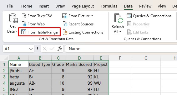
1. Select your range.
2. Go to the Data tab.
3. From the Get & Transform section, select From Table/Range.
   
4. If prompted, click OK in the Create Table pop-up.
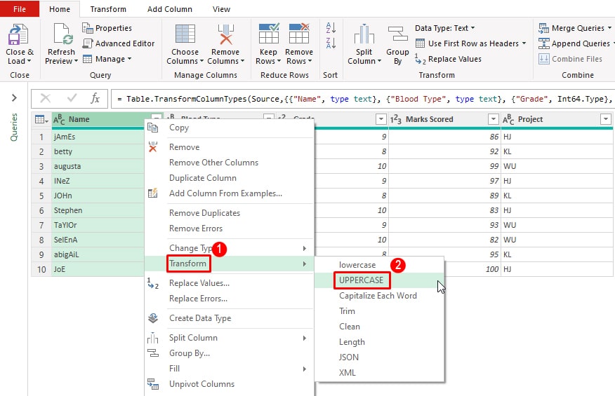
5. From the Power Query Editor, right-click on your column.
6. Select Transform > UPPERCASE.
   
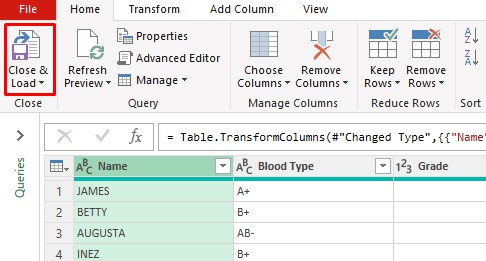
7. From the Home tab, select Close & Load.
   

Use Capitalized Fonts

If you don’t want to use formulas or go to Power Query to capitalize your fonts, you can simply use fonts that only use capitalized letters. There are a number of such fonts Excel offers by default so, you don’t have to download these fonts online.

Some of these default font names are Copperplate Gothic, Biz Udgothic, Castellar, Felix Tiling, The Serif Hand, and so on.

1. Select the texts from your spreadsheet.
2. From the Home tab, select the Font name from the Font section.
3. Scroll up or down to navigate through the library fonts.
   
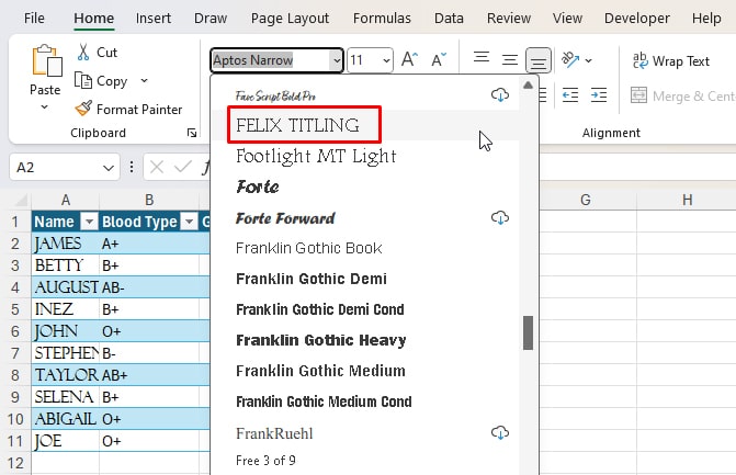
4. Once you find the best font, click on it to apply the font to your text.

Capitalize Letters in a PivotTable

You could realize the error in the casing of your letters after creating a PivotTable. As PivotTables aren’t directly editable, you may have issues capitalizing letters in them.

However, what you can do is change the case of the source table/range and then refresh your PivotTable to reflect the change. You can capitalize the source table/range using the UPPER function, then copy-pasting the results as values in the referenced fields.

Step 1: Capitalize Source Text

Use the UPPER function to capitalize the source text.

Step 2: Paste the Results as Values

1. Copy the formula results.
2. Select the referenced field and right-click on it.
3. Press V on your keyboard.
   

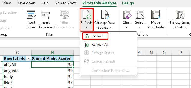
Step 3: Refresh PivotTable

1. Click on the PivotTable.
2. Go to PivotTable Analyze.
3. From the Data section, choose Refresh > Refresh.