Shading, oftentimes also referred to as highlighting, cells is a great way to make certain cells stand out. Excel offers numerous ways to shade a cell from your spreadsheet in a variety of colors. You can shade your cell to draw attention to a value, or purely for decorative purposes.
In this article, we will be covering the numerous ways you can shade one, or multiple cells in Excel. Additionally, we will also be discussing how you can set a criterion to shade a cell holding a select value in your spreadsheet.
Shade Cell Using a Background Fill
The quickest way to shade a cell is through the Font section in the Home ribbon. In this section, you will get the option to shade your cell with any solid color. Excel offers a list of library colors but you also have more color options.
- Select the cell you wish to shade. If you want to shade more than one cell with the same color, select the entire range.
- Head to the Home tab.
- In the Font section of the ribbon, select the fill icon.
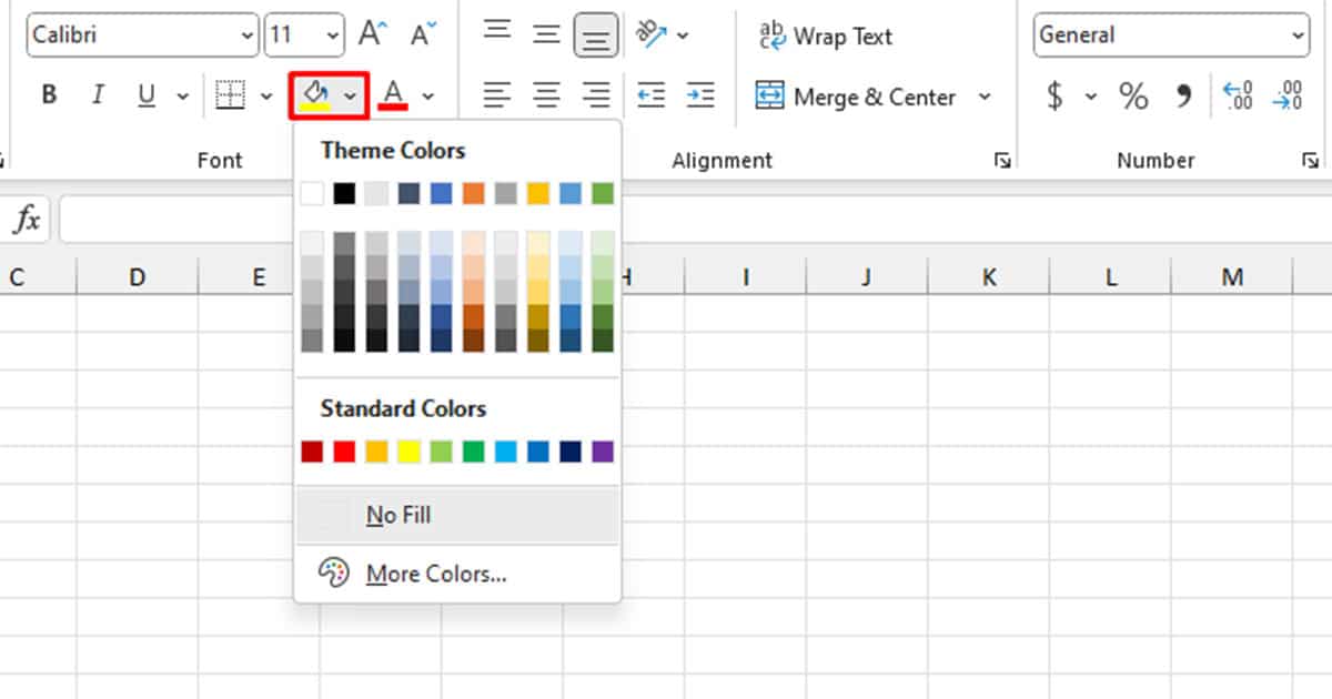
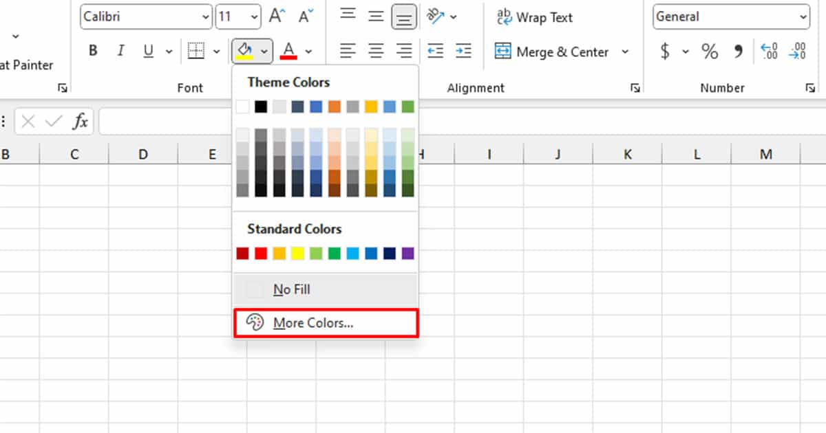
- Choose a color. If you do not see the color you wish to shade your cell with, select More Colors.
- Select your color from either the Standard or Custom tab.
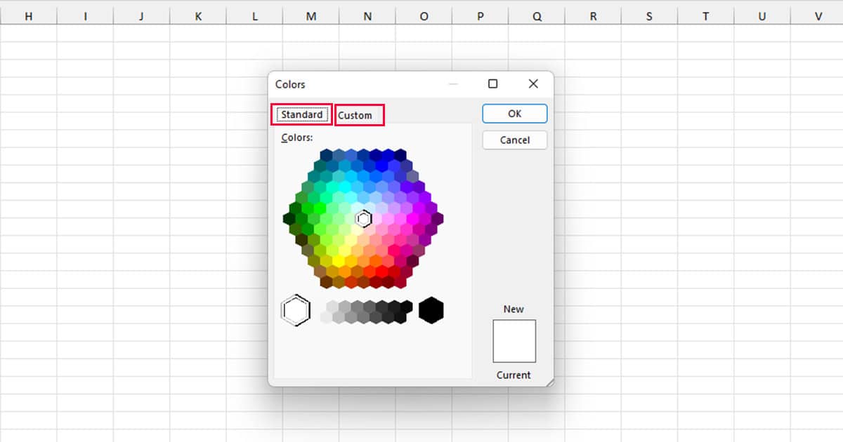
- Click OK.
Apply a Pattern to Shade your Cell
Excel also has the option to shade your cell using a pattern. You will get to choose from a range of patterns to shade your cell including customizing it with any color you desire.
- Head to the Home tab of your Excel program.
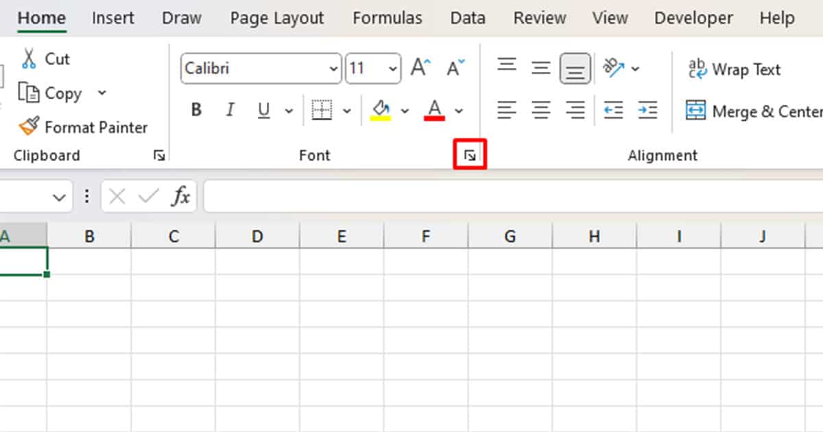
- Expand the Font section.
- Switch to the Fill tab.
- Under Pattern Color, choose a color for your pattern.
- Select the fly-out menu under Pattern Style to pick a pattern to shade your cell with.
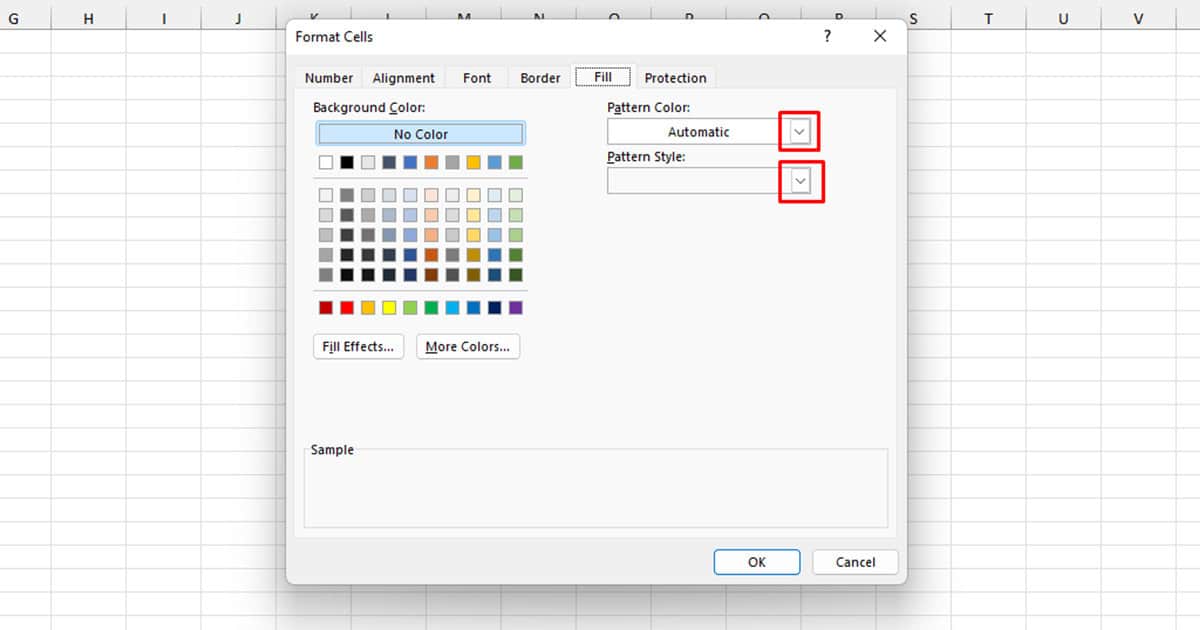
- Preview the pattern under the Sample section then click OK.

Shade Cell Using a Gradient
You can even apply a gradient in one or multiple cells in Excel. If you shade multiple cells with a gradient of colors, the gradient will be spread evenly across the cells. You can choose the number of colors you wish to use in your gradient, the shading style, and even the gradient variant.
- Select the cell or range you wish to shade.
- On your keyboard, use Ctrl + 1 to open the Format Cells window.
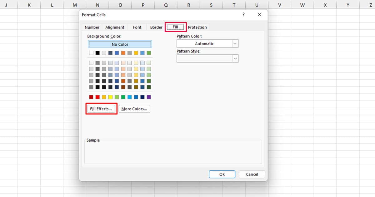
- Move to the Fill tab.
- Select the Fill Effects button.
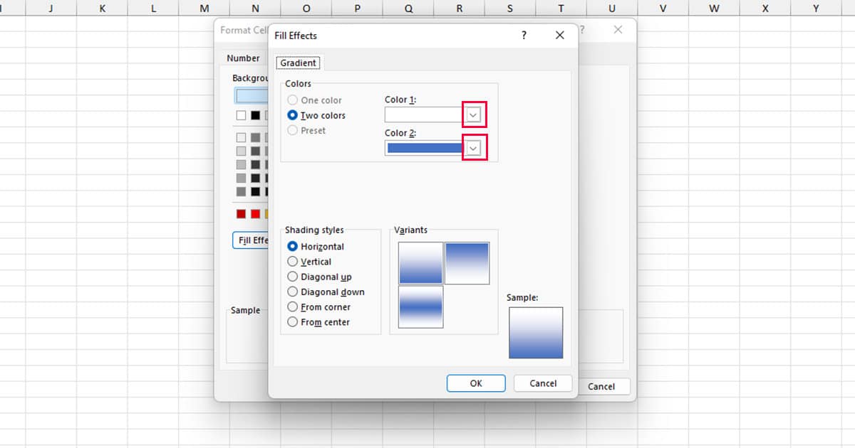
- Under Colors, pick the colors you wish to add to your gradient.
- Select a Shading Style.
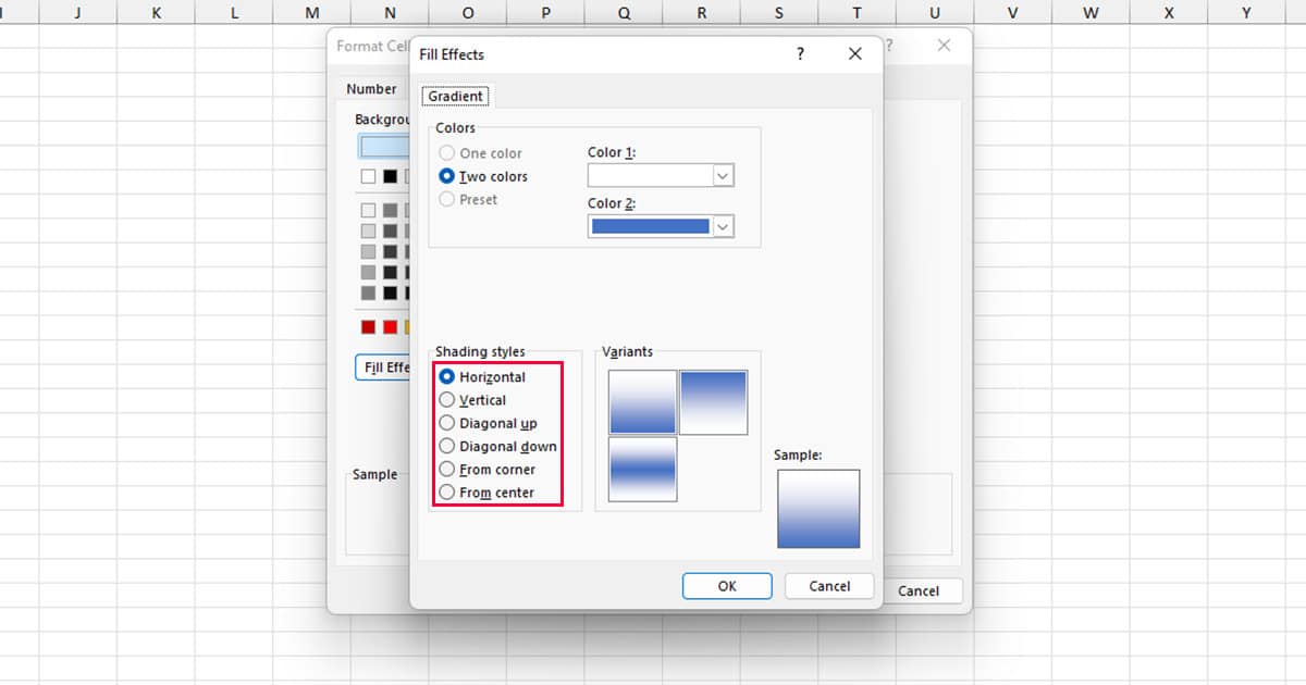
- Pick a Variant.
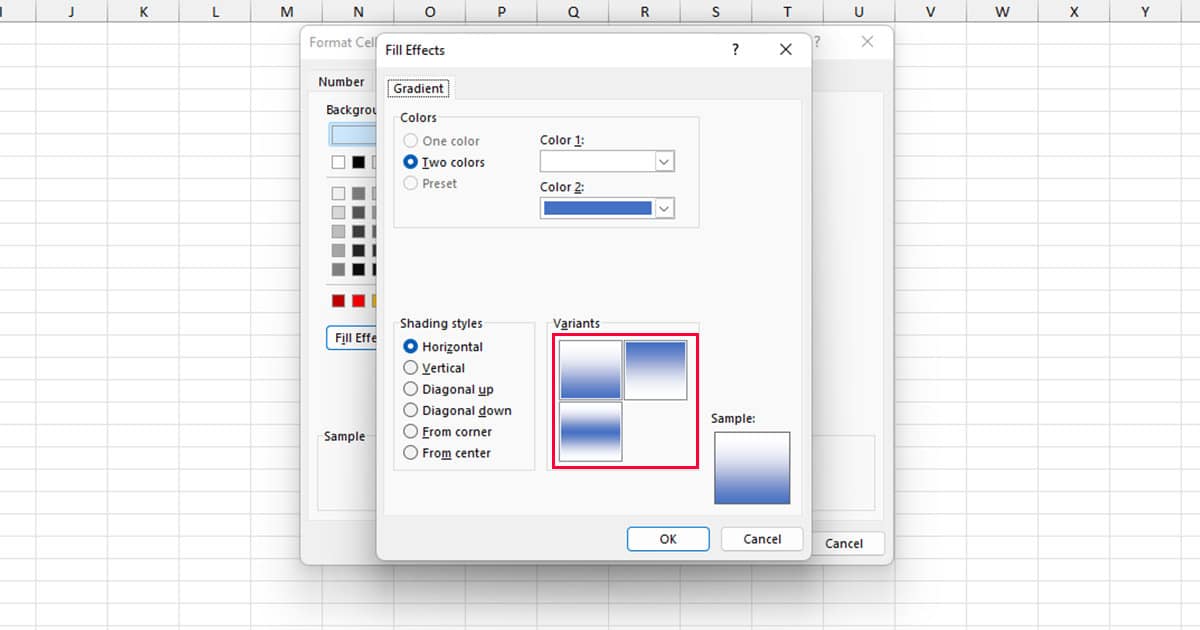
- Preview your gradient under Sample, and click OK.
How to Set a Criterion to Shade My Cell?
If you’re looking to shade your cell to emphasize cells holding a certain value, you should definitely consider using Conditional Formatting.
Conditional Formatting in Excel is a feature that allows you to format a cell that meets your set condition. Excel has a range of conditions including formatting a cell that a value greater, less than, or equal to a set value. There are other library conditions, including the option to enter a custom formula.
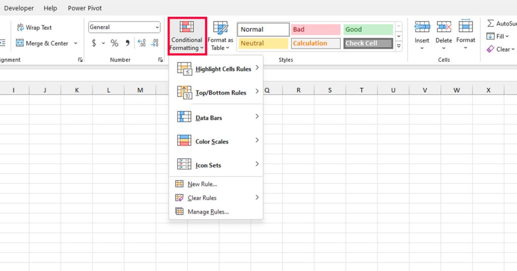
You can find the Conditional Formatting tool in the Styles section of your Home ribbon. You can choose from the numerous library Rules or create your own using the New Rule option.