Excel cell styling can make your worksheet visually appealing and, in some cases, help it stand out from the crowd. However, most professionals go overboard with it.
Inconsistent formatting, excessive color use, and overusing cell borders can have the opposite effect. The worksheet becomes cluttered, less professional, and unreadable.
If you are starting out on excel, I suggest you get your hands dirty with Excel’s Cell Style feature first. This has pre-formatted themes, headings, titles, and many more. You can experiment with these styles and even create your own Excel templates.
You can apply a default cell style, create your own, or import styles from other workbooks. Additionally, there are also format options to modify applied cell styles if needed.
Method 1: Apply Default Cell Style
Excel has a wide range of built-in cell styles in the Styles section of the Home tab. By default, each cell style has its own shade to represent the format. Depending on your need, choose and apply any one of them for your cell or cell ranges.
- Launch Excel workbook.
- Select Cell or Cell ranges.
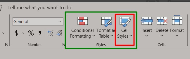
- On Home Tab, Go to on Styles section and click on Cell Styles.
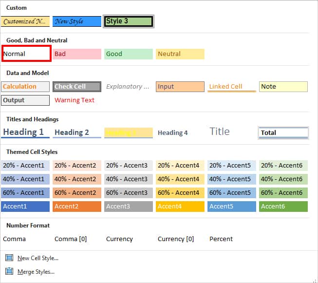
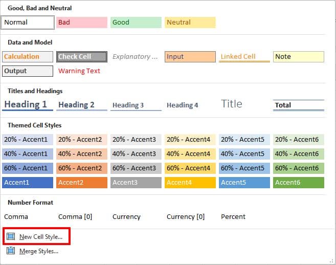
- Now, you can see 5 different categories of cell styles. Pick any one of them.
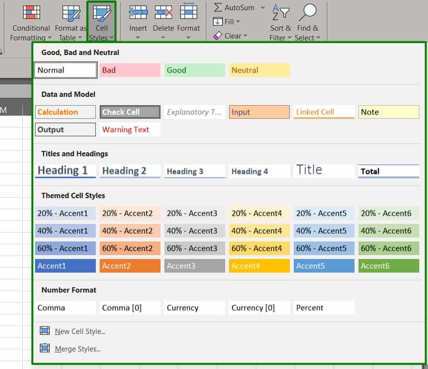
- Good, Bad and Neutral: In this style, you can see Normal, Good, Bad, and Neutral formats. Use these cell styles to represent whether a cell has positive or negative results at a glance. By default, Normal has no shade, Bad has a red shade, Good has green, and Neutral has yellow.
- Data and Model: Use Data and Model cell styles to define special cell values. Here, you can apply Calculation, Check Cell, Explanatory, Input, Linked Cell, Note, Output, or Warning Text.
- Titles and Headings: It includes cell styles like Heading 1, Heading 2, Heading 3, Heading 4, and Titles. Use this for your Row and Column Titles to make them stand out in your worksheet. Apply the Total style to indicate the output of data in a double underline.
- Themed Cell Styles: This style is mostly used to make your spreadsheet aesthetic and attractive. There are 5 different Accent styles. Apply any Accent to shade your cell or cell ranges with that color.
- Number Format: In this style, you can apply 5 number formats like Comma, Comma[0], Currency, Currency[0], and Percent. These styles are the same as the Accounting and Percentage styles of the Number group in the Home Tab. Use this for financial or any other numerical data.
Method 2: Create Your Own Cell Style
If you did not find the appropriate pre-built cell styles for your sheet, you can create your own cell style. Yes, you heard that right! Excel allows you to add a new customized style and apply them.
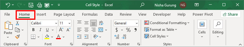
- On your worksheet, click Home Tab.
- Navigate to the Styles group and expand the Drop-down icon.

- Select New Cell Style.
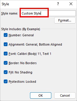
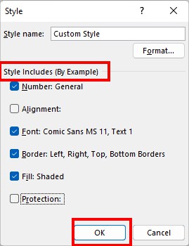
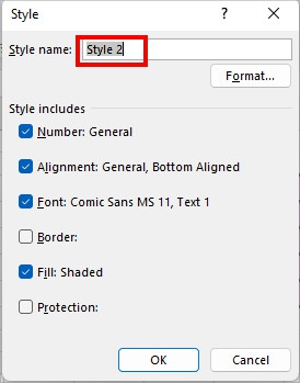
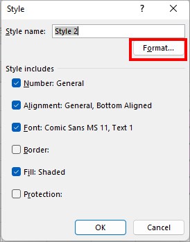
- A Style window will appear. On Style name, enter a Name for the cell style.
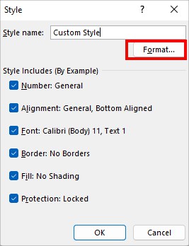
- Select Format menu.
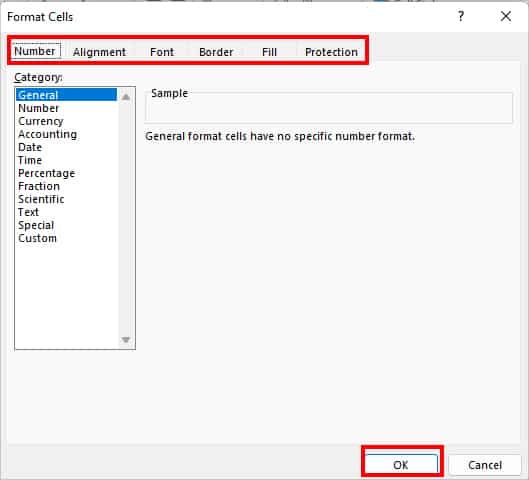
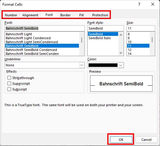
- On Format cells window, you can find the Number, Alignment, Font, Border, Fill, and Protection tabs. Go to each tab and select the Format you want to create. When done, hit OK.
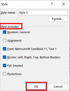
- Now, below the Style Includes (By Example), uncheck the boxes for the formatting to exclude them. Click OK to confirm.
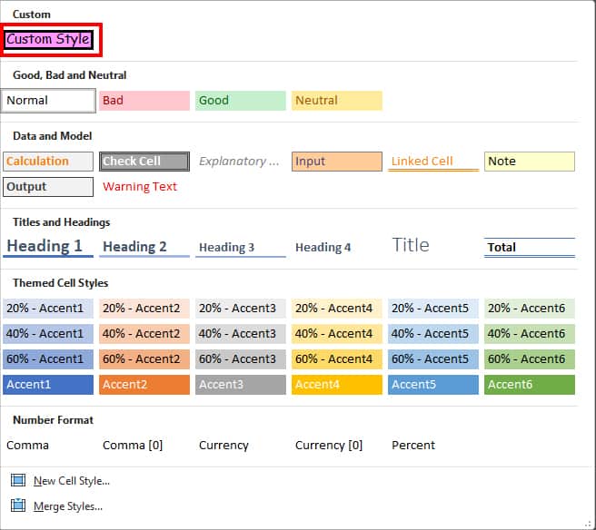
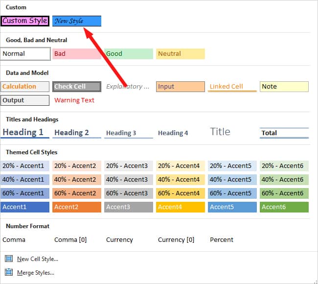
- To apply the the format, expand the More Icon in the Styles section.

- Under Custom, click on the Cell Style.
Method 3: Import Cell Style
Use this method if you already have a custom cell style in the other workbook.
With the Merge Styles command, you can import the existing cell styles from another workbook to your current workbook. It will copy all used cell styles of that worksheet.
You must note that one or more workbooks with a cell style must be open to use this command.
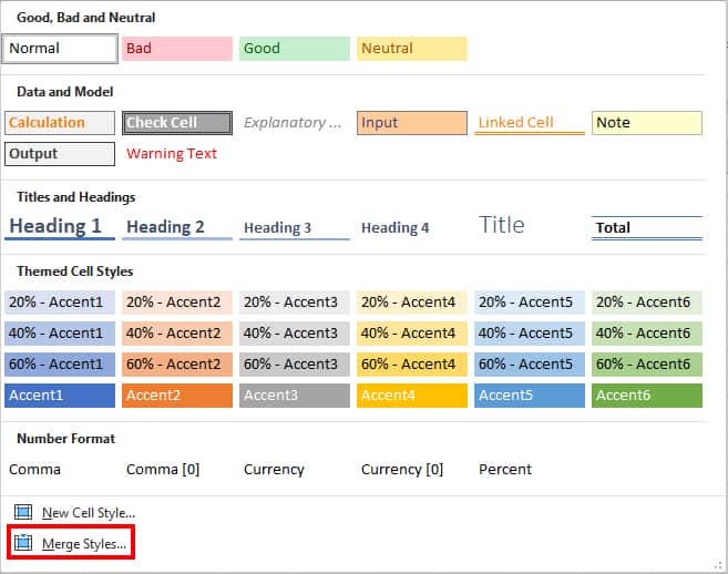
- On Home Tab, expand the Cell Styles menu.
- Select Merge Styles.
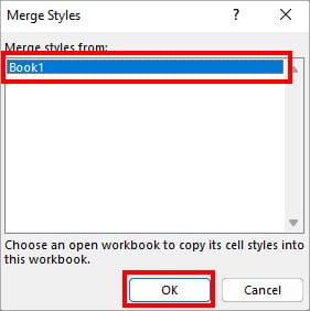
- On the Merge Styles window, choose a Workbook to import cell styles and click OK.
- In case the Cell Style name on both Workbooks is same, you’ll be prompted to choose Yes or No. ( Pick Yes to Replace and Pick No to have the same style)
- Again, go to the Cell Styles menu. Below the Custom menu, you should see the imported Cell Style. Click on the Style to apply.
How to Format the Applied Cell Style?
Once you’ve applied or created a cell style, you can also edit them. For this, you can find Modify or Duplicate option. Similarly, if you want to get rid of cell styles on your sheets, remove them anytime.
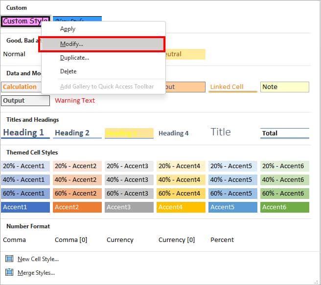
Modify Cell Styles
Use this menu to overwrite the cell style format like in the given picture.
- From Home Tab, hover over Styles group and click on More icon.

- Right-click on the applied cell style and pick Modify.
- On the Style window, retitle the Cell style.
- Click Format.
- In the Format Cells box, go to different tabs and set a Format. Hit OK to confirm.
- Below Style Includes (By Example), check or uncheck the boxes next to formatting to modify.
- Click OK.
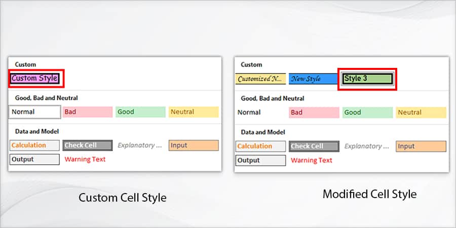
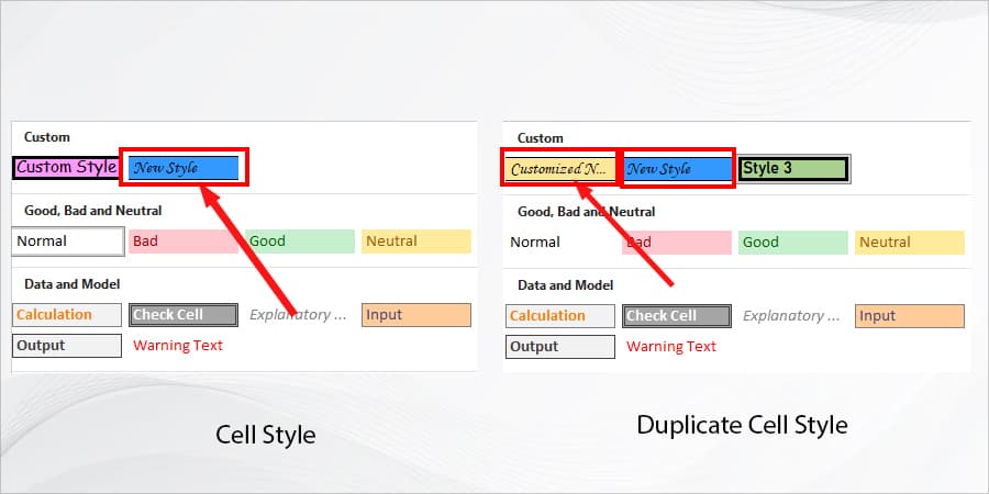
Duplicate Cell Style
You can also Duplicate your existing cell style instead of overwriting them. By doing so, you will have both cell style and modified cell style.
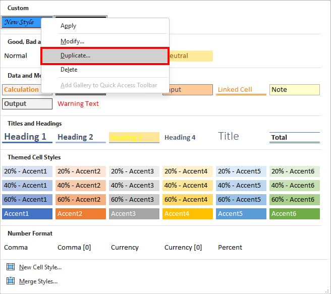
- Go to Styles Group of Home Tab. Then, click on the More Icon.

- Right-click on the applied cell style and select Duplicate.
- In Style name, rename your Cell Style. Then, click on Format.
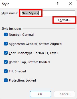
- In the Format Cells box, click on each tab and select a format to apply. Then, click OK.

- Below Style Includes (By Example), tick or deselect the boxes next to Formatting as per your wish.
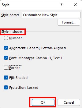
- Finally, click OK.
Remove Cell Style
You can get rid of the cell styles when you do not want them on your worksheet. Here, we are simply applying the Normal cell style to remove them.
- Select a Cell on your worksheet.
- On Home tab, navigate to the Styles section and expand the Drop-down icon.

- Below the Good, Bad, and Neutral menu, choose Normal.