How to Add Title to Chart in Excel

It is a standard format to include titles when creating a chart. This is so that anyone analyzing the chart knows what the illustration is based on. In Excel, if you do not reference the chart title with the dataset, Excel will simply enter “Chart Title” instead of your title as a placeholder.

In most cases, all you have to do is double-click on the placeholder text to edit the content and replace it with your actual Chart Tile. However, in cases you have accidentally deleted the text box, you will have to add the chart title from the Chart Design tab.

Insert Title As Chart Element

The Chart Title may be missing because you’ve disabled it as a chart element. Once you enable the Chart Title, Excel will insert either a placeholder text or the chart title if you’ve selected the data while creating the chart.

1. Select your chart.
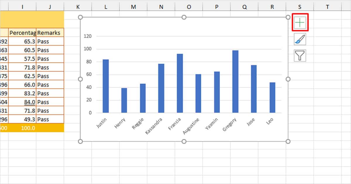
2. Click on the plus sign (+) on the right side of the chart.
   
3. Check the box next to Chart Title.
   
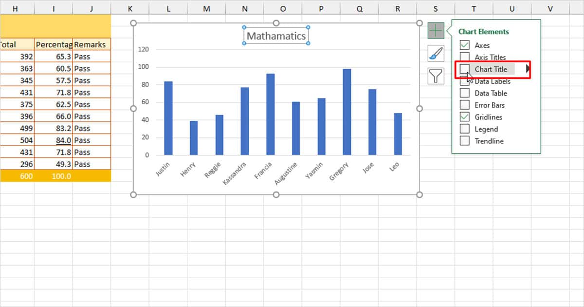
4. Double-click on Chart Title to edit the content.

Add Title from Chart Design

If you cannot see the placeholder text “Chart Tile” on top of your chart, you will have to manually enter the Chart Title from the Chart Design tab. The tab is only activated when you insert a chart on your spreadsheet. Select your chart then follow the following steps:

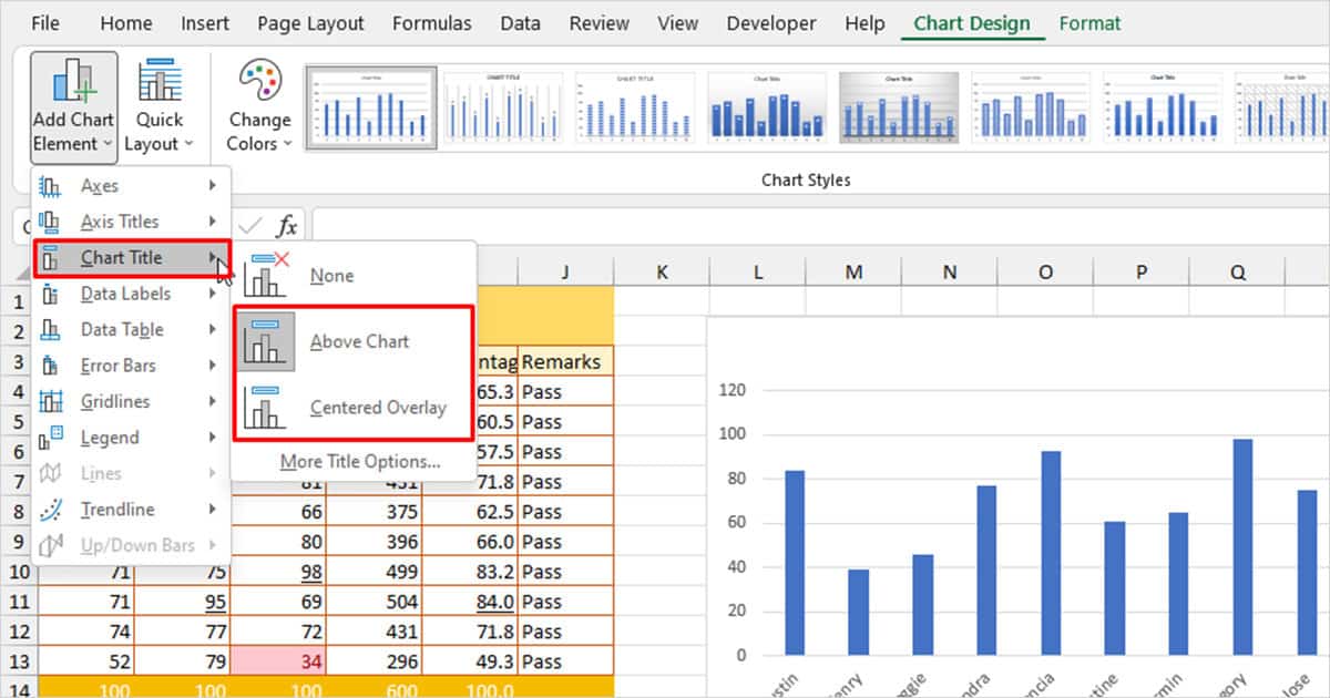
1. After you select your chart, head to Chart Design.
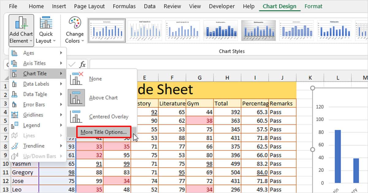
2. Click Add Chart Element > Chart Title.
3. Choose the placement of your Chart Title:

• Above Chart: The title will be placed on top of the chart.
• Centered Overlay: The title will be placed on the chart.
  

Include the Title in the Formula

You can make the process of inserting titles dynamic. When you’re referencing the data table to create a chart, include the text header. Whenever you change the title in the data table, Excel will automatically change the title on the chart.

Let me show you how this works using this data table. Let’s first create a table how we usually would. Head to Insert and select a chart. Right-click on the object and choose Select Data. 

In the Chart data range section, I entered this formula and hit OK:

=Sheet2!$A$3:$B$13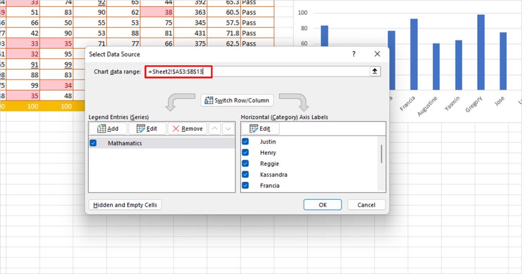

This formula references the data including the headers. As you may have noticed, I have spelled Mathematics incorrectly as “Mathamatics” in the table. To rectify this error, all I have to do is change the value in cell B3, which contains the Chart header.

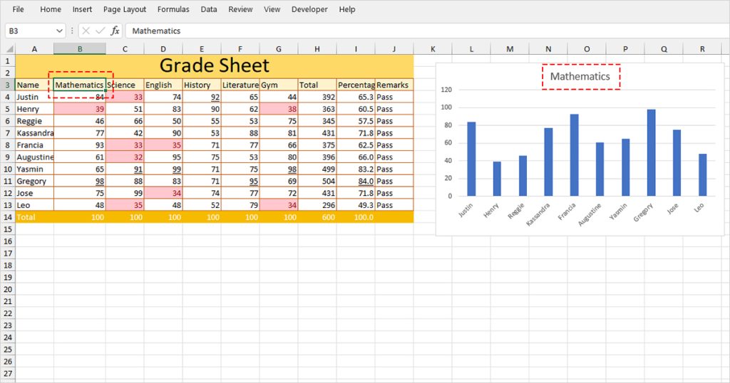
This is the best method to use to inset Chart Titles in Excel.

Change the Appearance of the Chart Title

You can customize the font and the formatting settings of the Chart Title.

Customize Font

You can change the font type, color, and effects of the font used as your Chart Title. Similarly, you can also adjust the character spacing of the text.

1. Right-click on your chart and select Font.
   
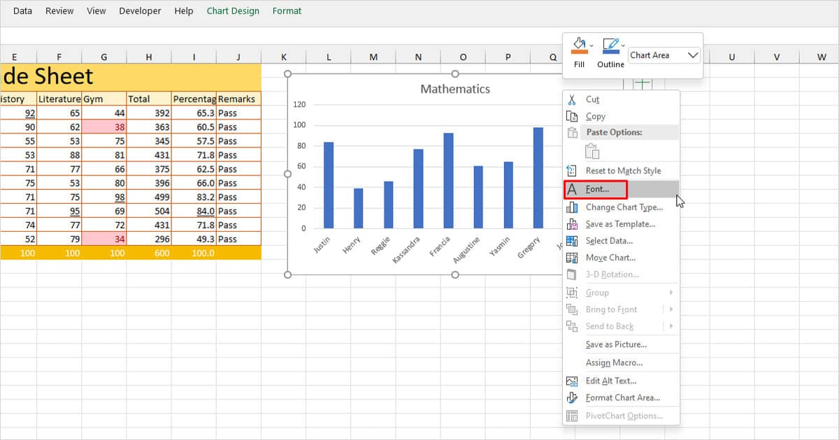
2. In the Font tab, customize the font type for Latin, Asian, and Complex fonts.
   
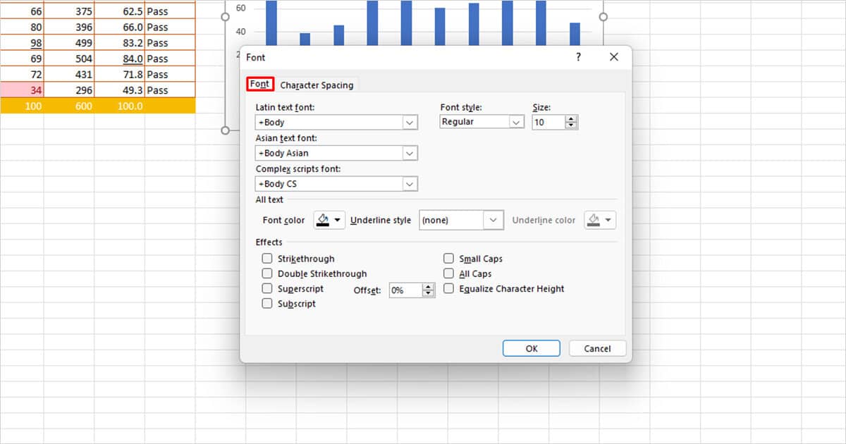
3. Adjust the style, and size under Font style and Size.
4. Under All text section, select font color, underline style, and color.
5. Select an option under Effects.
6. Head to the Character Spacing tab and select a Spacing.
   
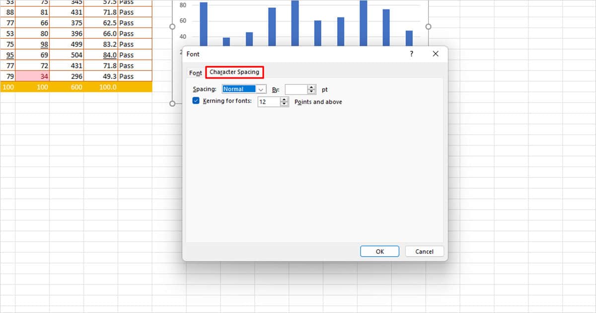
7. To apply Kerning after a specific text size, select the box next to Kerning for fonts and enter the text size.
8. Click OK.

Format Chart Title

You have the option to format the Title and the Text format of a chart’s title in MS Excel. This includes the color fill, effects, and size of both elements. Here are the steps you can follow to make these customizations:

1. Select your chart and head to the Chart Design tab.
2. Click on Add Chart Element > Chart Title.
3. Choose More Title Options.
   
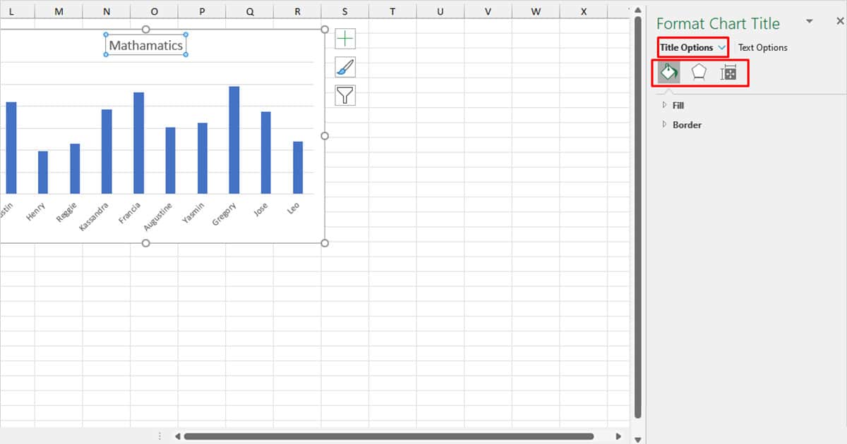
4. On the sidebar, select the icons under Title Options to switch between Fill & Line, Effects, and Size & Properties.
   
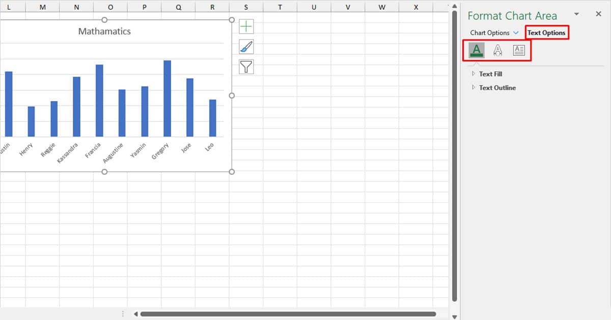
5. Switch to Text Options, and move between the icons to change the Text Fill & Outline, Text Effects, and Text Box.
   
6. After you’re done making the changes, select the cross icon on the top-right corner of the window to close the sidebar.