There are multiple Sorting options in Excel but today we’re talking about a distinct button to sort your data conveniently. You can simply click on it and choose how you prefer to sort your data. This is helpful when you’re lacking time or want to focus on only a particular data from your range. In this article, I’ve presented two effective and easy ways to add a Sort button in Excel.
Using the Filter Feature
The Sort button and the Filter feature synergize with each other to make sorting much more interesting. So, a quick and simple method to add a Sort button is by using Filter. Using this tool, you’ll get a specific drop-down arrow toggle on your column headings. You can then click on there and select how you want to sort. Here are the steps you’ll need to follow to do so:
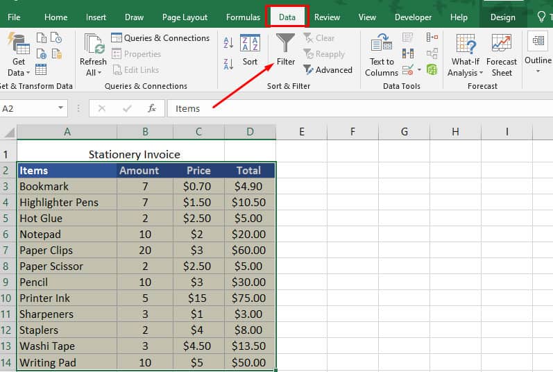
- Select the range of your data that you want to sort.
- Navigate to the Data tab above.
- Click on Filter.
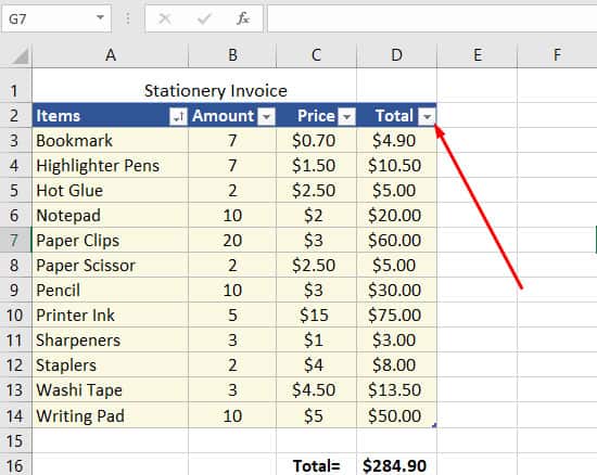
- Now, you can find the Sort button on the right of your column headings.
- Click on it and you’ll find various options, like Sort Smallest to Largest and vice-versa, color, number filters, and even a custom filter.
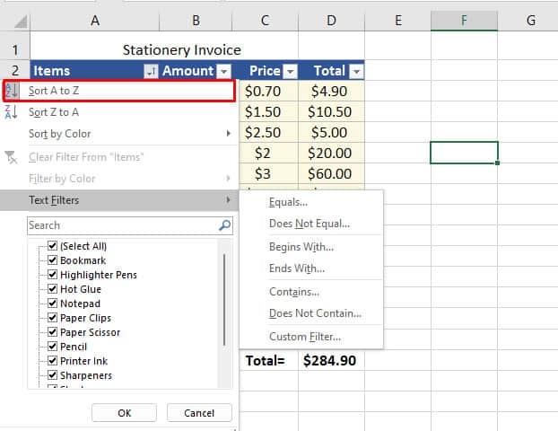
- Click on OK to exit.
Do remember that the sorting options will apply to all the selected range of data at once. Also, be careful when selecting the range because some data might remain inaccurate.
For e.g., I want to sort my ‘Items’ column alphabetically. If I only apply the Filter option to this single column, the changes will apply to it only. Whereas, its respective Prices column will stay inaccurate.
There’s also some flexibility while sorting your data. If you want to apply changes to only a few selected rows without deleting them, here’s what you can do:
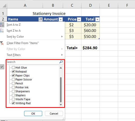
- Click on the Sort button.
- Below the Search option, you can observe all the rows that are selected and that the Select All button is also checked. Here, make sure to check only the rows that you want to sort. You can then uncheck the rest.
Using the Slicer Tool with PivotChart
The Slicer is a small tool that makes sorting your data easier. With your data using the Slicer, you can select only the column/row that you want to sort. Although this button won’t add a unique button to your existing data, you can sort the listed data directly from the Slicer window on the side.
As of the new update, you’ll need to open a PivotChart first and then only open the Slicer option from the Analyze tab of PivotChart tools. The PivotChart is an easy way to view or manage data as it offers a lot of flexibility. Using it, we can only choose to include a few selected columns without deleting them. The Slicer is its connected tool to pick which data to sort.
For the time being, we’ll ignore our initial data chart and focus on the new chart made by PivotChart. This is because any changes made to the Slicer will only display in the PivotChart. Here are the quick steps you can refer to:
- To create a Pivot Chart for our data, go to the Insert tab.
- Then, click on PivotChart.
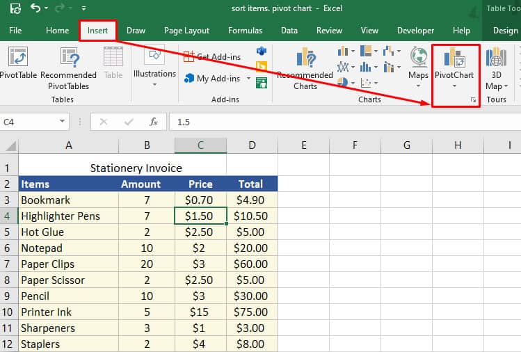
- A small window will appear. The first option asks you to select a table or range. You can either type in or directly select your range with the + cursor.
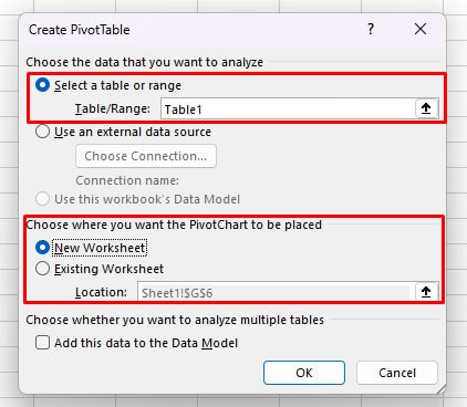
- Next, we’ll select where you want to place the PivotChart. In the Location option inside the same window, either select a new cell in the same sheet or select New Worksheet. Then, click on OK.
- You’ll now see the PivotChart Fields panel on the right. Below it, there are your column headings. Either check the boxes to select which column you want to sort or drag the columns to the different areas at the bottom. This will create a new chart for you.
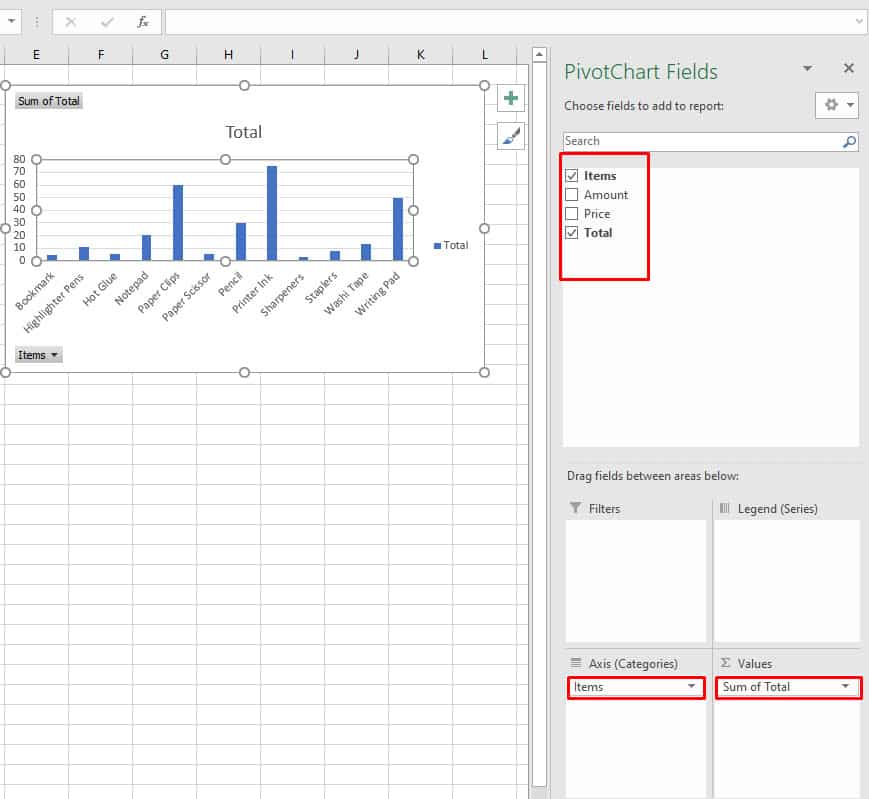 Here, I’ve selected only Items and Total to include in my chart. You can further customize this chart however you prefer. Next, we’re moving on to the Slicer tool.
- In the Tabs area, PivotChart Tools has additional tabs. Click on the Analyze tab and click on Insert Slicer. Select the columns you want to sort.
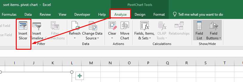
- Here, I’m selecting Items and Total only.
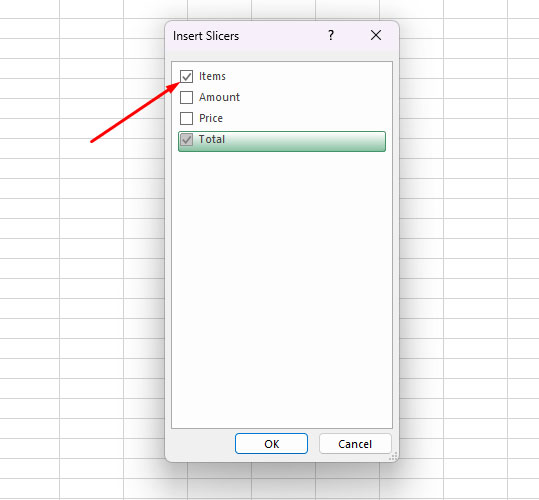
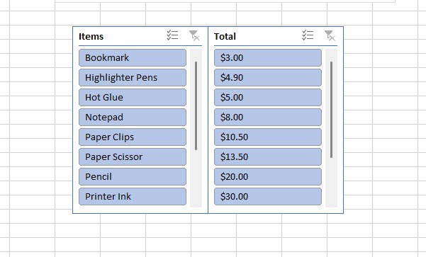
- There’s one Slicer for every column. So, here I have two Slicer tools for two columns. You can move them to the side for convenience. Now, select how you want to sort them.
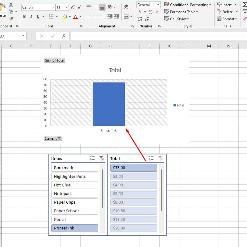
- What you select on the Slicer tool, the PivotChart will only display it and its corresponding data. So, you won’t need to select the respective data in all the other Slicers. For e.g., I only want to select Printer Ink data. Now, the tool will automatically only select its related cost in the Total column. Similarly, my PivotChart is displaying the selected data only.
- To select multiple data, hold CTRL and continue clicking on any data.
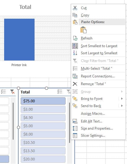
- To further sort the data, right-click on the Slicer and select your sorting options. Alternatively, you can also check the table in the top-left corner. Click on its Sort button and select Label Filters or Value Filters.
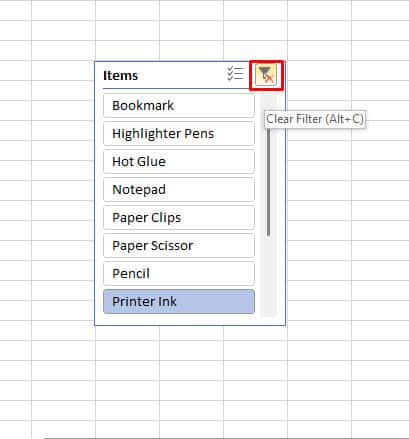
- To remove the filters, click on the Clear Filter icon.
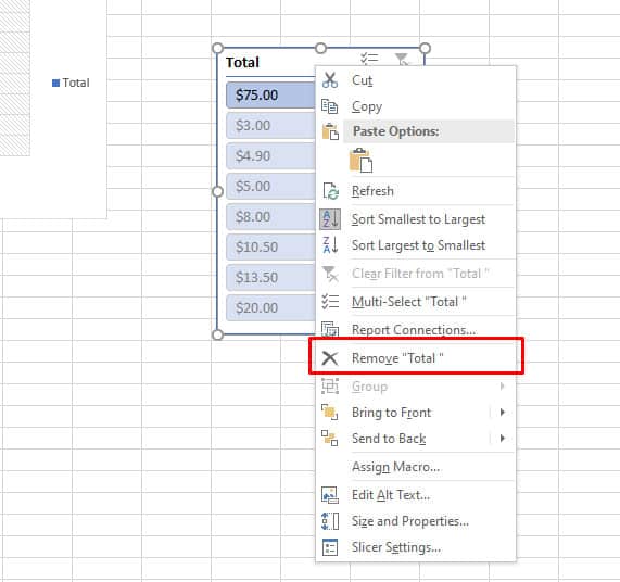
- If you want to delete a slicer, right-click on it and then click on ‘Remove <column name>.’
