In Google Sheets, you may often find yourself adding numbers to calculate the sum. For Instance, it could be to find out the monthly total expenses, student’s test scores, total sales, shopping bills, solve statistical problems, and many more.
Usually, most beginners would use the (+) plus sign to add two numbers just like in maths or calculators. But, I do not recommend using this arithmetic operator in Sheets as it can extremely tedious and overwhelming. You wouldn’t want to spend your whole day summing up the numbers manually.
Well, Sheet has various SUM functions dedicated to adding values in different circumstances. So, you can smartly use functions such as SUM, SUMIF, SUMPRODUCT, SUMSQ, and DEVSQ to perform additions.
Using Add Function
Google Sheets has an Add function which is just the formula version of the (+) operator to sum two numbers. So, instead of using the plus sign, you can simply input values in the formula for quick calculation.
Syntax: ADD( value1, value2)Add function accepts only two values as function arguments. If you attempt to input 3 or more values, it’ll result in a #N/A error. So, use this function only if you have to add two numbers. You could use the numbers or cell references in this function.
Let’s say you need to add numbers 7 and 3. For this enter the formula as
=ADD(7,3)
or,
=ADD(A1, A2)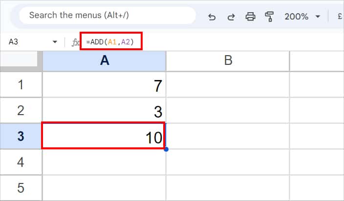
It’ll return the 10 as an output.
Using SUM Function
ADD function has its limitations of not accepting more than two arguments. So, if you need to add a series of values or cell ranges, use the SUM function. Google Sheet’s SUM function returns the total sum of sequential numbers or cells.
Syntax: SUM(value1, [value2,...])Function Arguments:
- value1: number or cell range you want to add
- value2: extra number or cell ranges you want to add
This function is built to accept up to 30 arguments at maximum. However, as per Google Sheets, you can enter an arbitrary number of arguments.
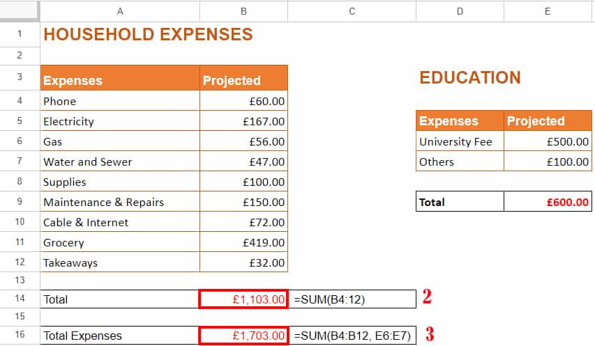
Let’s assume, I need to find out the Total projected value of Household Expenses. There are three ways I can use the SUM function to calculate the value. Take a look at the examples in the given table.
| SN | Examples | Formula | Result | Description |
| 1 | Sum each number | =SUM(60,167,56,47,100,150,72,419,32) | 1103 | Here, the SUM function takes up number 60 as value 1, 167 as value 2, and so on to add. |
| 2 | Sum cell ranges | =SUM(B4:B12) | 1103 | Adds all the values from cells B4 through B12 and returns the total. |
| 3 | Sum non-sequential cell ranges | =SUM(B4:B12, E6:E7) | 1703 | The formula takes cell B4:B12 as value 1 and E6:E7 as value 2. Then, returns the sum of both cell ranges. |
Using SUMPRODUCT Function
For some calculations like Weighted Averages, you’d have to multiply the numbers first and add them together for the final output. But, in Sheets, I suggest you use the SUMPRODUCT function to calculate the outcome at once.
SUMPRODUCT function returns the total sum of product numbers from the same array or cell ranges.
Syntax: SUMPRODUCT(array1, [array2,....])Here, array1 refers to the cell ranges or array you want to multiply. Similarly, array 2 is the extra cell ranges to multiply.
Let’s suppose, you have the Product name in Column A, Quantity in column B, and Costs in column C. Now, you need to calculate the total cost. For this, use the formula mentioned in the box.
=SUMPRODUCT(B2:B7, C2:C7)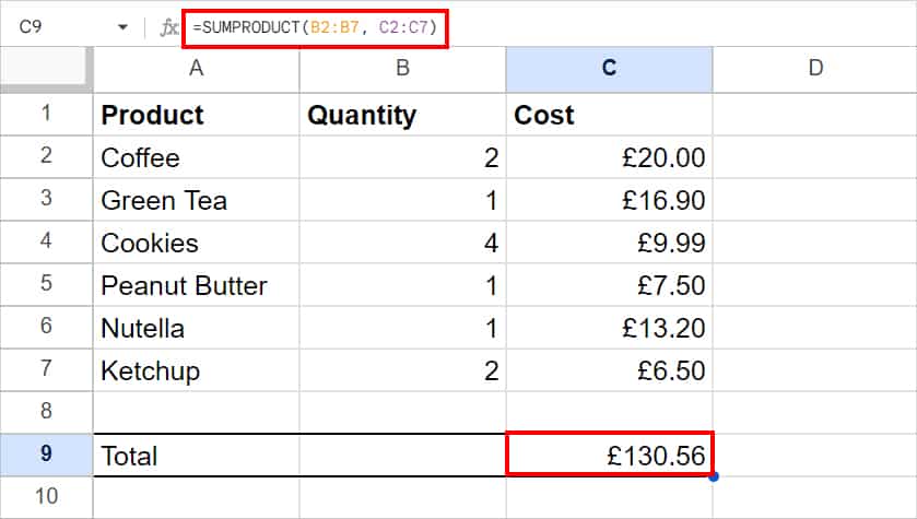
We have passed down two arrays in the formula. Here, the formula will calculate the product of cells (B2 * C2) + (B3 * C3) + (B4 * C4), and so on. Then, return the total sum of 130.56.
Using SUMIF Function
There can be instances where you might want to add numbers based on a condition. For example, add only numbers greater than 10. During such cases, you can use the SUMIF function.
The SUMIF function returns the conditional sum of numbers from a cell range.
Syntax: SUMIF(range, criterion, [sum_range])The SUMIF function takes up the following arguments.
- range: Cell ranges to apply criteria.
- criterion: Specify the condition for the sum
- If your range has text values, your criteria should be a string. You can use wildcard characters (?, *, ~) in the criteria.
- If your range has numbers, your criteria can be number or string. You can use operators (=, <, >) to set the greater than, equals to, and lesser than criteria.
- sum_range: Cell ranges to sum.
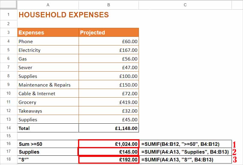
Suppose, I have a list of Household expenses with the projected costs. Now, to get the conditional sum results, I will apply several criteria. Check out the table for more details.
| SN | Criteria | Formula | Output | Description |
| 1 | Sum Expenses greater than or equals to 50 (>=50) | =SUMIF(B4:B12, “>=50”, B4:B12) | 1024 | Here, B4:B12 is the range to apply the criteria. Since we have specified “>=50” criteria, it’ll exclude the values less than 50 while summing the numbers from the B4:B12 range. |
| 2 | Sum “Supplies” | =SUMIF(A4:A13, “Supplies”, B4:B13) | 145 | In the formula, we’ve passed down the “Supplies” criteria from cells A4 through A13. Similarly, our sum range is from B4 through B13. Hence, it’ll sum only the values of Supplies and return the output. |
| 3 | Sum all the Expenses starting with the letter S “S*” | =SUMIF(A4:A13, “S*”, B4:B13) | 192 | Here, we have passed down “S*” criteria for cells A4 through A13. Our sum ranges are B4 through B13. So, the formula will sum all texts starting with S. |
Using SUMSQ Function
If you need to calculate the squares of numbers and add them together, there is a SUMSQ function in Google Sheets. In most cases, it could be to solve statistical problems. SUMSQ function returns the total sum of squares in cell ranges.
Syntax: SUMSQ(value1, [value2,...])SUMSQ function takes the following arguments.
- value1: Initial number or cell ranges to sum squares.
- value2: Extra number or cell ranges to add to value1.
Let’s take an example. Say you need to sum up the square numbers of 3, 5, 6, and 7. For this, you can enter the formula as
=SUMSQ(3, 5, 6, 7)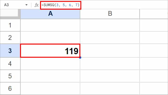
The above SUMSQ formula will calculate (3*3) + (5*5) + (6*6) + (7*7). Thus, you’ll get 119 as a result.
Using DEVSQ Function
Some users might find the need to add the squared deviation numbers to analyze the variance in a stock price index. Or, to check the variance in temperatures. For this, Google Sheets has made it easier to calculate the sum in one go. Sheet’s DEVSQ function returns the sum of squared deviations from the sample.
Syntax: DEVSQ(value1, [value2, ….])Here, the DEVSQ function takes up only two arguments which are the cell ranges to sample.
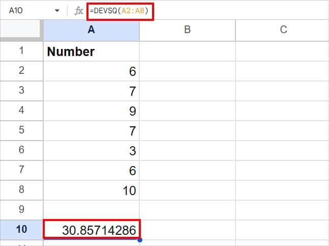
Example: Let’s suppose, you need to calculate the sum of given numbers. For this, you can simply enter the formula as
=DEVSQ(A2:A8)