When you have a larger data set, analyzing a specific group of data can be a bit complicated. For example, if you’re looking at the sales list of a company, you may want to filter the data to check the list of employees who generated the least amount of revenue. Fortunately, Excel has the Filter tool for you to locate such values.
Asides from the tool, you can also use the FILTER function in Excel. You can use both of these methods for basic to advanced filtering of your data.
Using the Filter Tool
The Filter tool in Excel covers almost all basic data filtering. This includes filtering your data on the basis of cell values, and color, and even setting rules for numbers.
If you convert your range to a table (Ctrl + T), Excel will automatically insert the filter option. You can also add a filter on a normal data range through the Excel ribbon or an Excel shortcut.
Shortcut:
Ctrl + Shift + LRibbon:
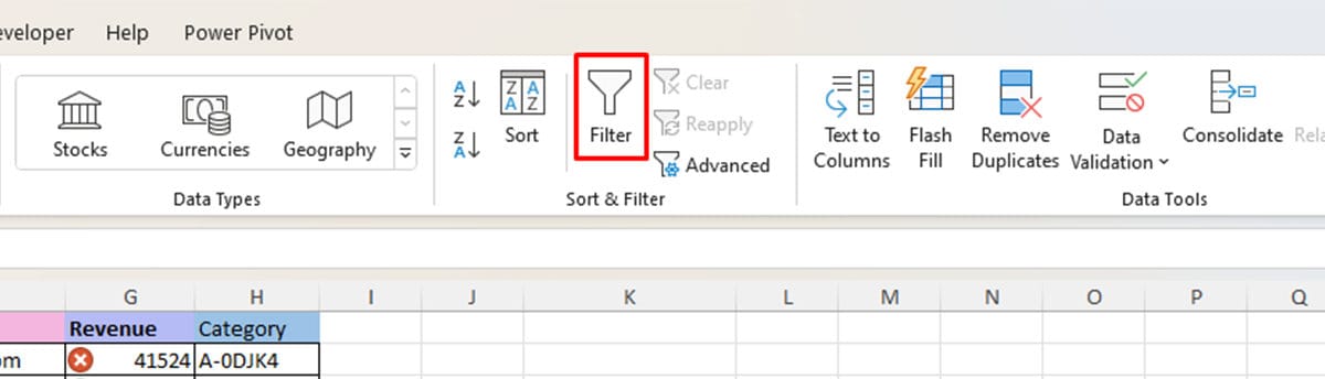
- Head to the Data tab.
- Click on Filter from the Sort & Filter section.
Filter Range by Cell Values
Cell values are almost always the criteria used to filter a data range in Excel. Once you add a filter to your range, you will find a drop-down menu on the top cell of a column. You can filter by one, or multiple criteria.
- Select the drop-down icon from the header of the reference range.
- Uncheck the box next to Select All.
- Enter your criteria in the search box or click on the box next to them.

- Click OK.
Filter by Color
Filtering through color is a great filter option especially if you’re using conditional formatting. You can also use this method if you’ve applied conditional formatting icons on your cells.
However, it is not limited to conditional formatting. Even if you’ve manually changed the fill color, or the font color you can use these criteria to filter by color in Excel.
- Select the fly-out menu on the column header.
- Choose Filter by Color.
- Select your criteria.
Filter by Numbers
This filter option can be a lifesaver for documents like sales sheets. The filter feature has the option to filter your data set through multiple rules, including the option to create your custom filter.
- Click on the filter menu on the reference column header.
- Select Number Filters.
- Choose your criteria.
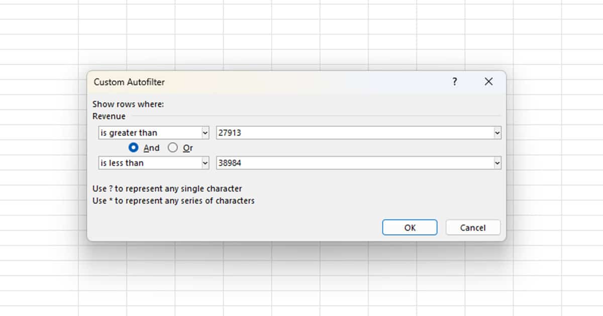
- If you wish to create a custom filter, select Custom Filter.
- Click on the fly-outs or enter custom values in each field.
- Select OK.
Use Advanced Filter
Excel also offers an advanced way of filtering your data set. Using advanced filters, you have more control over setting the criteria range to filter your range. You can also use an advanced filter to filter duplicate data from your table.
Before you use the advanced filter, you must first create a criteria range. This range should include the reference column header followed by your criteria under it. You can have one or multiple criteria depending on your needs.
We have included four different examples in this section for you to see how advanced filter works in Excel.
Example 1: Filter Data According to One Criterion
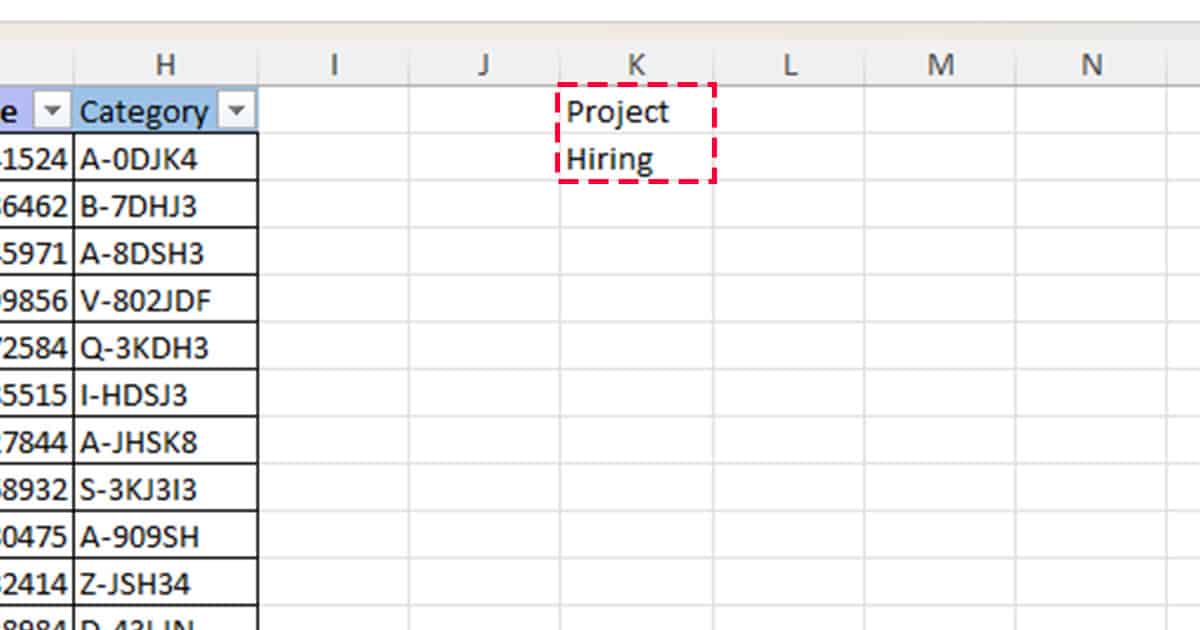
Let’s start with the basics. We will be using the advanced filter tool to filter our data set according to Project. Excel will remove the data of all employees except the ones working on the Hiring project using the filter tool.
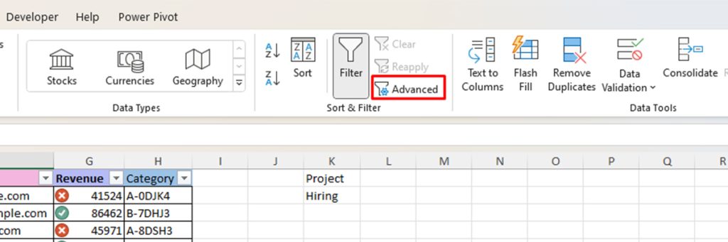
- On an empty cell, enter “Project”. Immediately under Project, enter “Hiring”.
- Head to Data and select Advanced from the Sort & Filter section.
- Choose whether you want to filter the range on the same or different location under Action.
- Reference your data set in the List range field.
- Set your criteria range.
- Click OK.
Example 2: Filter Data According to Multiple Criteria
To filter your data set according to multiple criteria, all you have to do is to set two fields as your criteria range. You can set multiple criteria to filter cells within the reference column or set multiple reference columns.
We will be filtering our data set according to the Name, Jared, and Status, Active.
- On two empty cells, enter Name and Status next to each other.
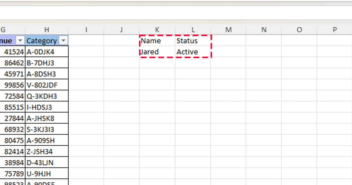
- Under Name, enter Jared, and under Status, enter Active.
- Move to Data and choose Advanced.
- Choose whether you want to filter the range on the same or different location under Action.
- Reference your data set in the List range field.
- Set your Criteria range.
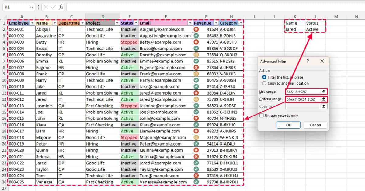
- Click OK.
Example 3: Set Multiple Filter Criteria for the Same Column
You can choose more than one criterion to filter data within the same reference column. For this, you will have to enter your criteria under the same criteria range.
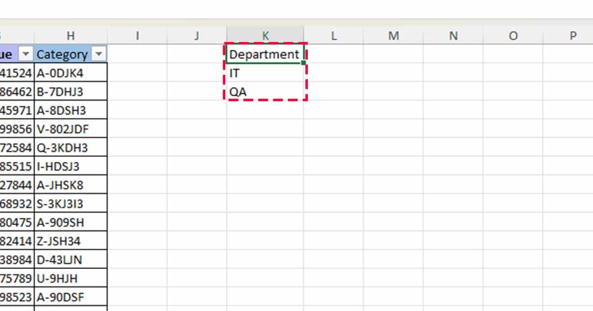
We will be using the same table as before to set two filters only those values with IT and QA under the Department column.
- On a new cell, enter Department.
- Right under the cell, enter IT then QA.
- Head to Data > Advanced.
- Next to List range, reference your data set.
- Reference the new Department column as your Criteria range.
- Click OK.
Example 4: Use Wildcards to Filter Data
The use of wildcards is one of the key features of advanced filters. You can use the asterisk, question, and tilde wildcards under the criteria range to filter your data set accordingly.
Here’s a little reminder of what each of these wildcards does in Excel:
| Wildcard Name | Symbol | Function |
| Asterisk | * | Select all values that begin or end with the set value. *ly can return both sly and ally. Similarly, Un* can return both unhappy and unhinged. |
| Question | ? | Acts as a placeholder for the missing text. T?m can return both Tim and Tom. |
| Tilde | ~ | Overrides the function of a wildcard when used in front of them. ~*ly return *ly and ~t?m returns t?m. |
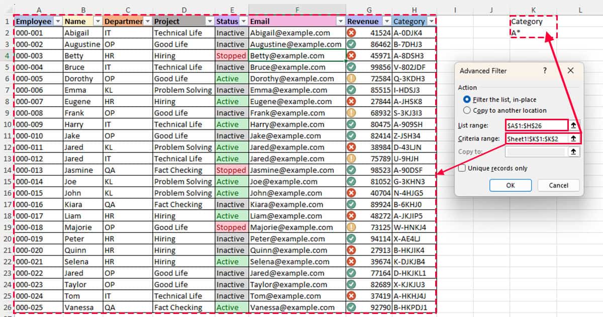
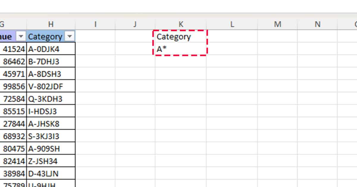
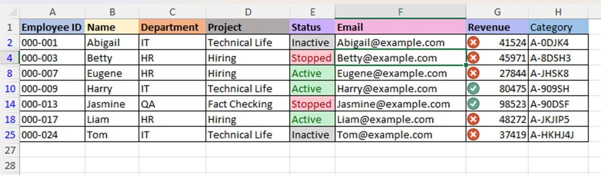
Let’s use the asterisk wildcard to filter data to view only those fields that start with the letter “A” in the Category section.
- Create a criteria range. Under “Category”, enter A*
- Head to Data > Advanced.
- Choose an Action.
- Select your data range as the List range.
- Next to the Criteria range, reference the new field you just created.
- Click OK.
Use FILTER Function
Excel also has the FILTER function to set multiple criteria for filtering a data set in your worksheet. You can use the FILTER function as an alternative to using the Advanced Filter tool.
Here is how you can use the FILTER function while constructing a formula:
=FILTER(array, include, [if_empty])- array: Your data set
- include: The criteria for filtering data
- [if_empty]: Message if the data specifies in “include” isn’t found
Example 1: Filter by One Criterion
Let’s use the FILTER function to filter out all data except IT from the Department column. Here is what our formula will look like:
=FILTER(A1:H26,C1:C26=“IT”)
Example 2: Filter by Multiple Criteria
By default, FILTER only takes in one criterion to filter data. However, you can use the BOOLEAN login to set multiple criteria. Simply, concatenate as many criteria as you want using the asterisk (*) operator.
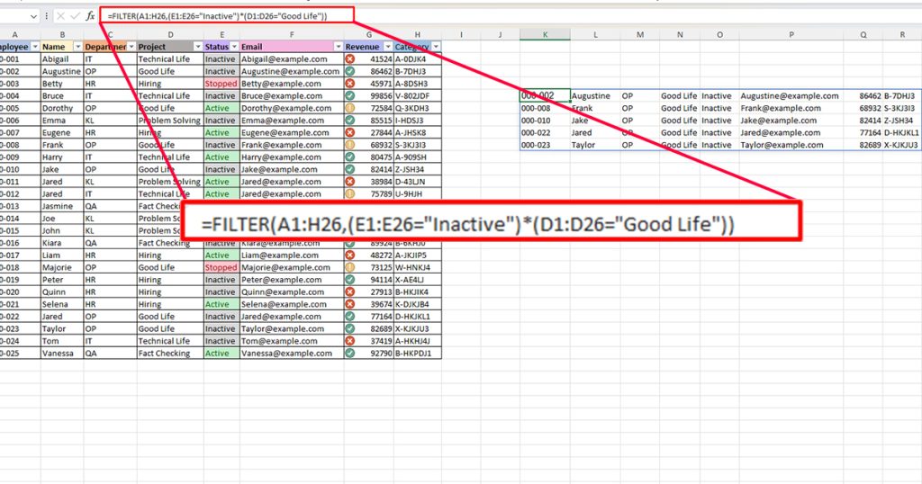
We will use FILTER to extract data whose Status is Inactive, and is under Project, Good Life.
=FILTER(A1:H26,(E1:E26="Inactive")*(D1:D26="Good Life"))