HLOOKUP is a powerful lookup function in Excel that retrieves values from different rows in the same column. HLOOKUP is mainly used during data analysis in Excel worksheets.
HLOOKUP is similar to VLOOKUP. The only difference between them is that HLOOKUP looks up values horizontally, while VLOOKUP retrieves values from different columns in the same row. However, the arguments used in both of these functions are quite similar.
What is HLOOKUP?
HLOOKUP basically means horizontal lookup. In larger data sets, you can use this function to check the values that are in different rows of the same column. HLOOKUP works by moving horizontally to look for the set reference. Then, it moves down the row according to the row number you’ve set in the arguments.
You can use the HLOOKUP function in all versions of Excel.
Arguments Used in HLOOKUP
HLOOKUP takes in four arguments as its arguments. Among these, three are required while one is optional. Here is how you need to arrange the arguments while constructing a formula using the HLOOKUP function:
=HLOOKUP(lookup_value,table_array,row_index_number,[range_lookup])| Argument | Data Type | Description |
| lookup_value | INTEGER | The reference value. Remember to only reference a cell from the first row |
| table_array | RANGE | The table with your data |
| row_index_number | INTEGER | The row your value is in |
| [range_lookup] | BOOLEAN | Enter TRUE (1) for an approximate match and FALSE (0) for an exact match. |
Application of the HLOOKUP Function
You can use HLOOKUP in different ways to extract different values. Similarly, you can also use tools like Data Validation to make HLOOKUP dynamic. In this section, we will be looking into diverse ways you can use HLOOKUP in your worksheet.
Example 1: Use HLOOKUP to Return an Exact Match
In this example, I will show you how you can use HLOOKUP to return the exact. You can use this method when you’re sure about the data you’re entering in the “lookup_value” section. If your lookup value has any time of typo, HLOOKUP will return the #N/A error.
Let’s use the HLOOKUP function to return the marks obtained by Frank in Physics in this mark sheet. As we know for sure that the header we’re going to reference is Physics, we can pass this lookup_value as the exact match.
Here’s how we have constructed the formula using the HLOOKUP function to return us the marks scored by Frank in Physics:
=HLOOKUP(“Physics”,A1:F11,6,0)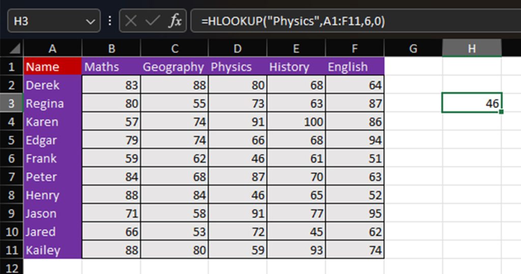
Example 2: Use HLOOKUP to Return an Approximate Match
Sometimes, the exact value you’re looking to get the result for does not really exist in the table. This is mostly true for tables with numerical values. In cases like these, you can use HLOOKUP to approximately match your value. You can do this by entering “FALSE” or “0” in the range_lookup section.
HLOOKUP will look for the value that is smaller than the look_up value that you’ve provided. If the lookup_value is smaller than the smallest value in the table_array, HLOOKUP will return the #N/A! error.
In this table, we have a lab report of 5 different chemicals. Each column represents the temperature each chemical was put under and if they were reactive or not. For instance, chemical B was not reactive between 0.20-0.29 but was reactive at 0.30-0.39 unit temperature.
To see if Chemical A is reactive at temperature 0.54, we will be using the HLOOKUP function in the following format:
=HLOOKUP(A9,A1:J5,2,1)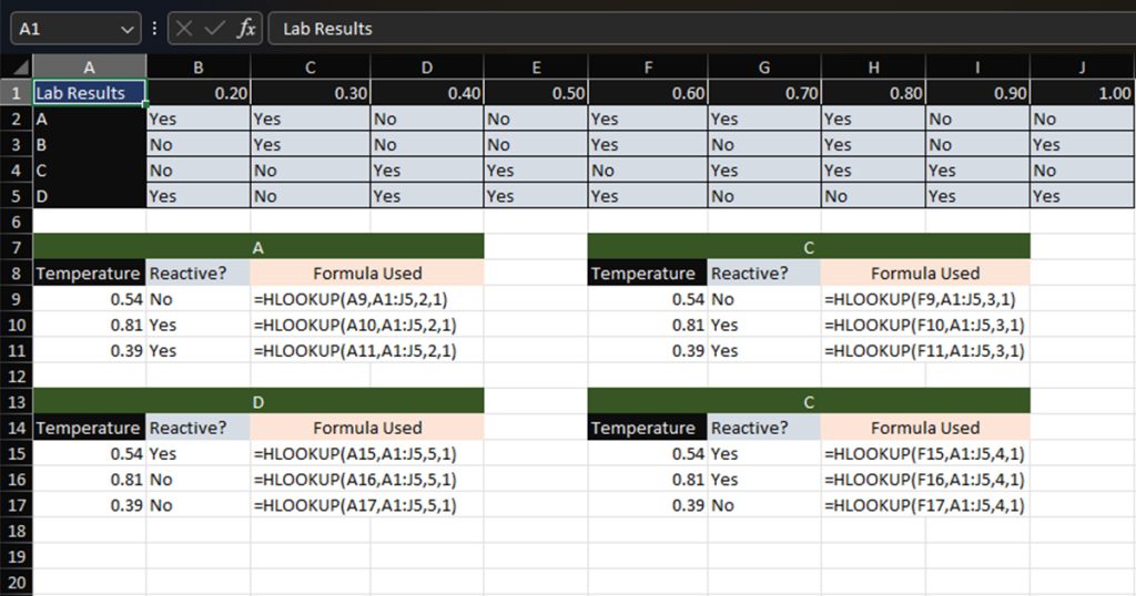
I entered two other conditions and used the HLOOKUP function to generate the results.
Example 3: Using Wildcards in HLOOKUP
There are certain times when you might not be sure about the lookup_value. While you can always do an approximate matching in HLOOKUP, you can also use wildcards. You can use wildcards, including asterisk (*), question mark (?), and tilde (~) to create the lookup_value. You will have to do an exact match when using wildcards.
| Wildcard Name | Symbol | Description |
| Asterisk | * | You can use Asterisk to look up all values that start or end with the entered letter. |
| Question Mark | ? | You can use the Question Mark symbol as a placeholder symbol for missing texts. |
| Tilde | ~ | You can use Tilde when you don’t want asterisks and question marks to act as wildcards. |
Here is a data table. Imagine this table has more columns; possibly hundreds. Now, while analyzing the data, your co-worker told you they’re not sure if they’ve entered “Amount” or “Total Amount”. You obviously cannot use exact matching in this case, but, you also cannot use approximate matching as it will end you up with the #N/A error.
Let’s use wildcards to resolve this issue. Here’s how we constructed the HLOOKUP formula using the asterisk (*) wildcard:
=HLOOKUP("*"&A13,A1:F11,6,FALSE)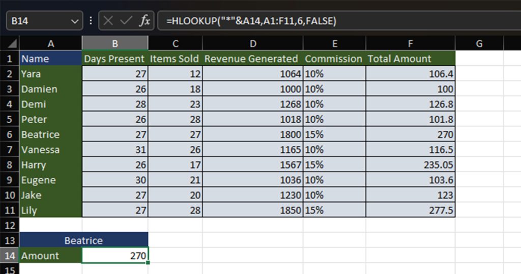
Use Data Validation to Make HLOOKUP Dynamic
Let’s go back to example 1. Let’s assume we now want to see the marks scored by Frank in History. You will have to manually change the lookup_value from “Physics” to “History”. While you could do it once or twice, it can get tedious after some time.
Let’s save you the hassle, shall we? Instead of hardcoding our value, let’s use cell referencing. Now, every time you change the data in the cell, your lookup_value changes. To make this process feel even more automated, let’s create a drop-down list using data validation to switch between our data.
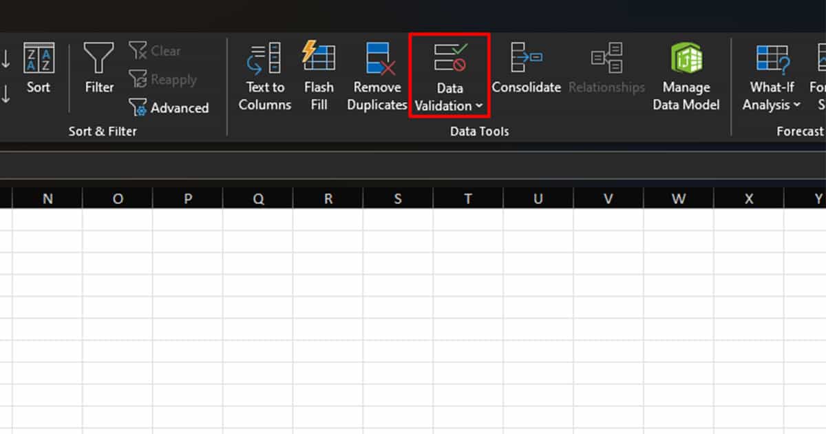
- Head to the Data tab from the menu bar.
- From the Data Tools section, select Data Validation.
- In the Settings tab, select the fly-out under Allow > List.
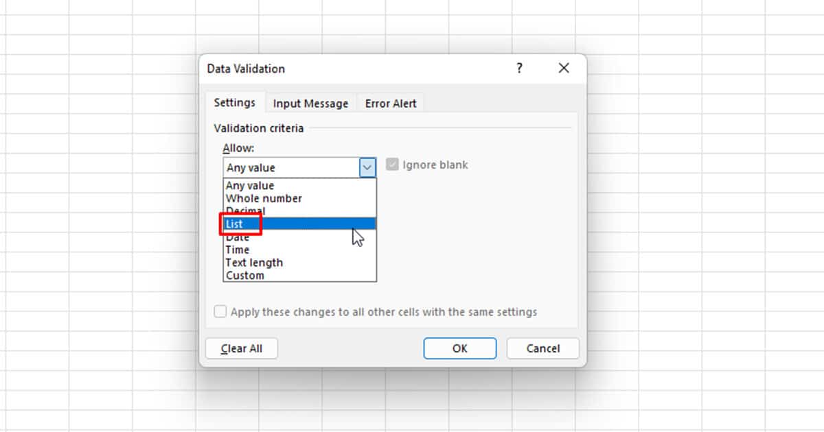
- Collapse the window under Source and select the range B1:F1.
- Click OK.
Now, every time you need to switch your lookup_value, you can click on the fly-out menu next to the cell and select your data.