How to Highlight Every Other Row in Excel?

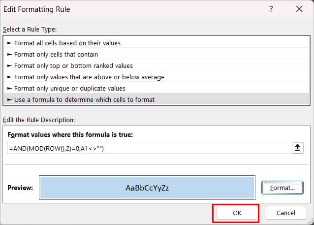
It can be hard to scan data when you have a large spreadsheet in Excel. Imagine having to locate the value of every Tuesday from the following data. You are left squinting through the rows and rows of drudgery. What a nightmare!

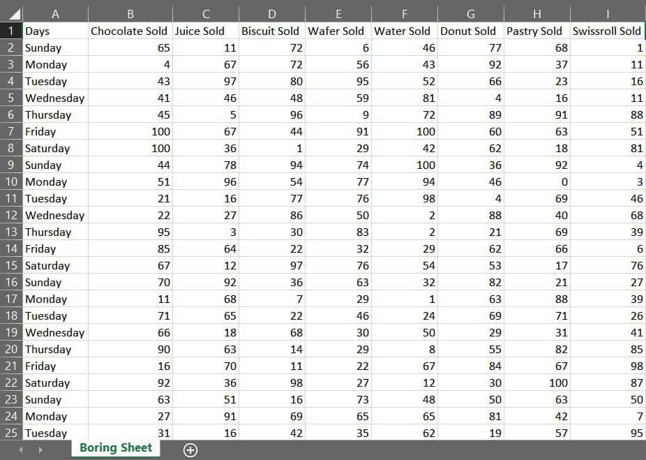
Luckily, there is an option to highlight every other row and make it more readable. This can help you find information at a glance. For this, you can use the following two approaches:

Format Data as Table

This is the quickest and most simple way to highlight rows. Excel offers a wide variety of table designs with alternate shaded rows. You can select from these templates or opt for the default option.

If you are looking to highlight data just for aesthetic purposes and don’t care if it is in table format, this method is best for you. As Excel has pre-built table styles, you do not need any formula for this approach. 

Tables are dynamic, so whenever you add extra rows, Excel will automatically highlight them too.

To change to table format,

1. Launch Excel.
2. Go to your Worksheet.
3. Highlight the cells and navigate to Home Tab. 
   
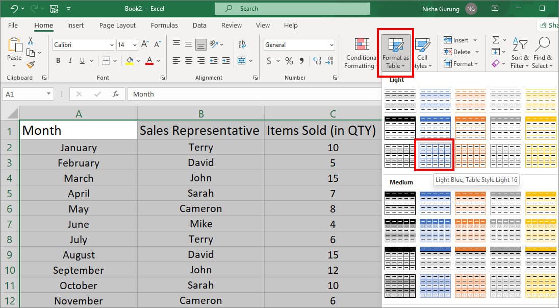
4. On Styles menu, click on Format as Table. Then, choose a Table style with alternate row highlights. 
   
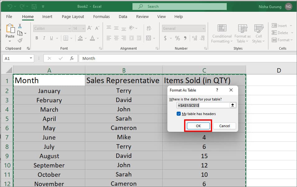
5. Check the box for My table has headers. Pick OK to confirm. 
   
6. To change the highlight colour, select a cell and go to Table Design tab. 
   
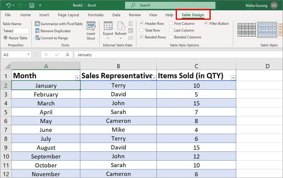
7. Pick a colour from Table Styles. 
   

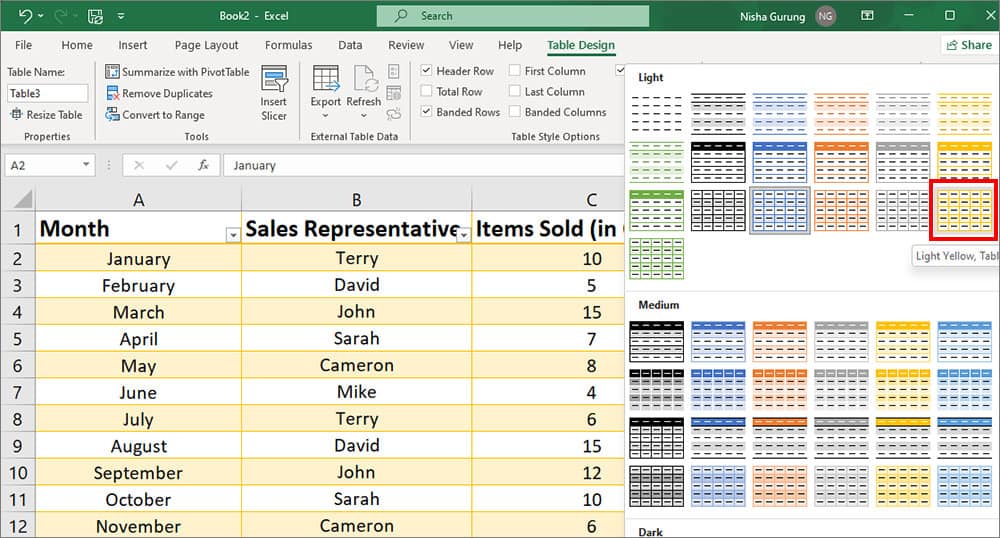
Quick Tip: In case you want to get rid of table format while keeping highlights, convert the table to a normal range. For this, navigate to Table Design > Convert to Range. Note that when you do this, you will no longer get automatic highlights after adding rows. 

Use Conditional Formatting

Conditional Formatting is one of the best tools to shade rows or columns based on different conditions. For Instance, shade every row with the name “John” or value “less than 10” in your worksheet.

You can use this feature especially to draw attention to specific data. In this method, we will use formulas to highlight rows depending on each format rule.

Every Alternate Row

To highlight every alternate row, we will use the MOD ROW formula in Excel. This formula will check whether the rows are odd or even and apply shades accordingly. 

Let’s see how this formula works with an example first.

Case 1 [Highlights every alternate even rows]

=MOD(ROW(),2)=0  

In this condition, when you divide each row by 2, you get 0 as a remainder. So, it will identify even rows and shade them only. 

For example: =MOD(ROW(4),2)=0 (4 is divisible by 2. So, we will get 0 as the remainder)

Case 2  [Highlights every alternate odd rows]

=MOD(ROW(),2)=1

In this condition, when you divide rows by 2, you will get 1 as the remainder. It means these are odd rows. So, Excel will find the odd rows and highlight them.

For Example: =MOD(ROW(3),2)=1 (3 is not divisible by 2. So, we will have 1 as the remainder)

Now, you can use one of the given formulas to highlight every alternate even or odd row. Here’s how you do it.

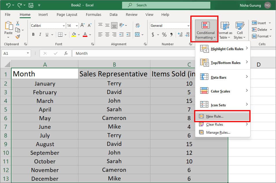
1. On your worksheet, highlight the cells to format. Then, go to Home Tab.
   
2. Click on Conditional Formatting > New Rule.
   
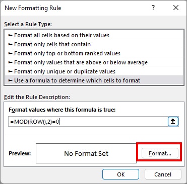
3. On New Formatting Rule box, pick Use a formula to determine which cells to format. 
   
4. Then, enter formula =MOD(ROW(),2)=0 or =MOD(ROW(),2)=1.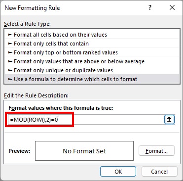
   
5. Click on Format.
   
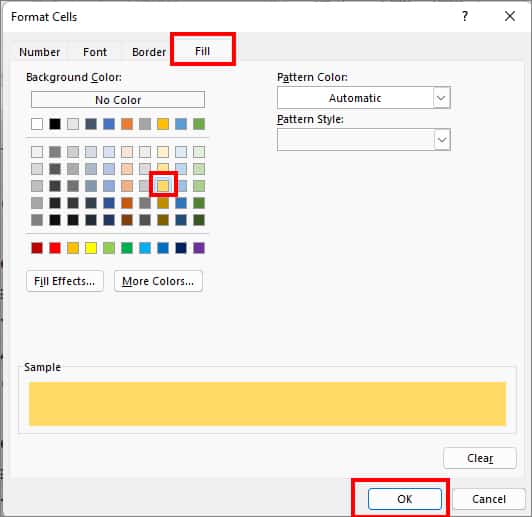
6. Navigate to the Fill tab and pick a Colour to highlight. Then, click on OK. 
   
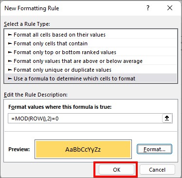
7. Again, click OK.
   

Every nth Row

It’s more easier to find the exact cell ranges when you highlight every nth row in your spreadsheet. We will again use the MOD ROW formula to apply this condition. However, this time, we will add cell values to the formula. 

As a reference, we have provided an example to highlight every 3rd or 5th row below.

1. On your worksheet, highlight the cells to format.
2. Go to Home Tab.
   
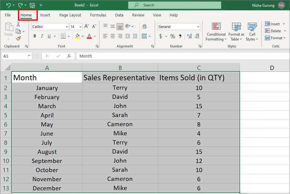
3. Click on Conditional Formatting > New Rule.
   
4. On New Formatting Rule box, pick Use a formula to determine which cells to format. 
   
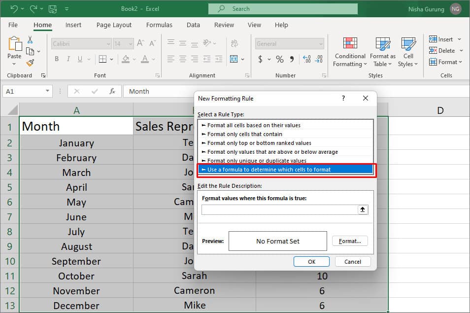
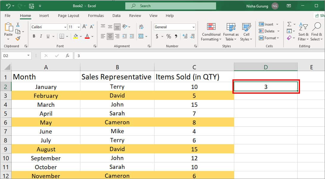
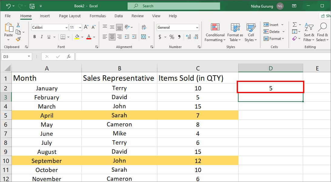
5. On Formula bar, enter =MOD(ROW(A2:C2),$D$2)=1 (For A2:C2, highlight the first rows and remove dollar signs. For $D$2, click on the empty cell.)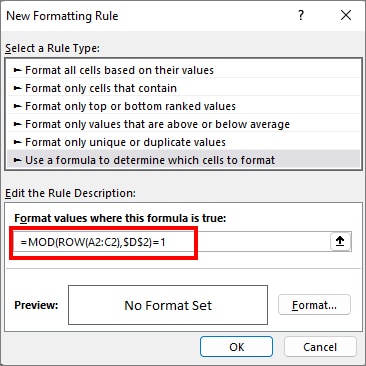
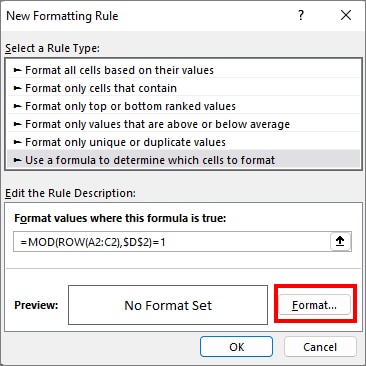
6. Select Format.
   
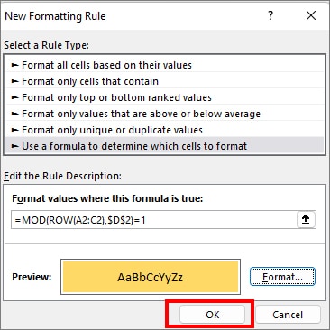
7. On Fill tab, click on Colour and hit OK.
   
8. Again, pick OK to confirm.
   
9. On the D2 cell, enter 3. It will highlight every 3rd row. 
   
10. Similarly, if you enter 5, it will highlight every 5th row. 

Every Row Based on Text

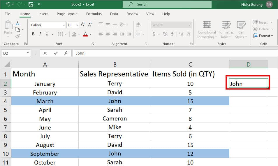
Sometimes, you would want to highlight entire rows based on a specific text to retrieve data. For example, highlight every row with the name “John.” There is a different rule to apply this condition. 

Here’re the steps for it.

1. On your worksheet, select all ranges. Then, go to Home Tab.
   
2. Click on Conditional Formatting > New Rule.
   
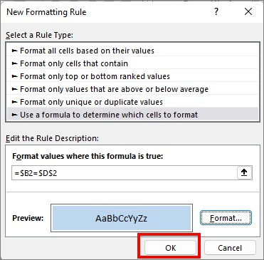
3. Click on Use a formula to determine which cells to format. 
   
4. Enter =$B2=$D$2. (For $B2, Highlight the first cell of the column with text and remove the $ sign before 2. For $D$2, Select any empty cell.)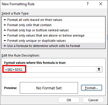
   
5. Choose Format.
   
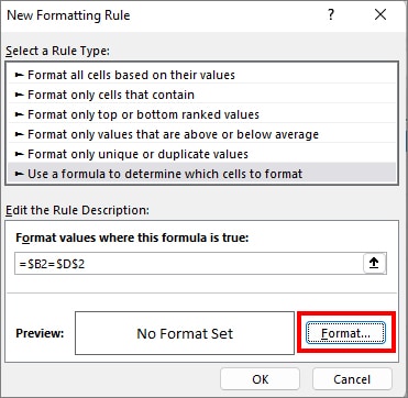
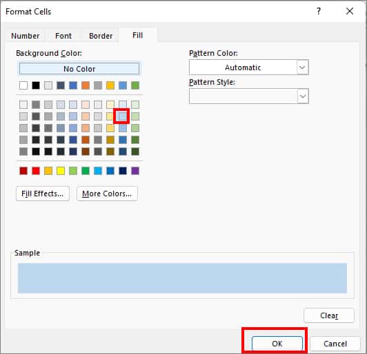
6. Pick a Colour and choose OK.
   
7. Again, select OK. 
   
8. Hover over D2 cell. Type a Name to highlight and press enter. 

Every Row Based on Number

You can also highlight rows based on the number. It can come in handy when you have to select the end results and analyze them.

Let’s assume, you have to find a value that is less than 10 in these steps.

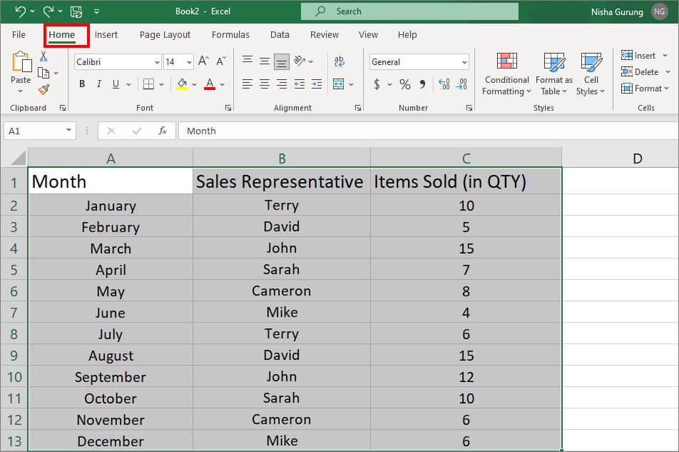
1. On your worksheet, highlight all ranges and click on Home Tab.
   
2. Navigate to Conditional Formatting > New Rule. 
   
3. Select Use a formula to determine which cells to format.
   
4. Enter =$C2>10 . (For $C2, select the first cell with number value. You can replace number 10 with any value.)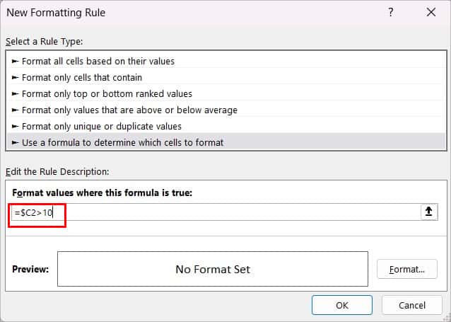
   
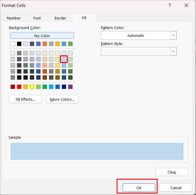
5. Click Format and select colour to highlight. Choose OK.
   
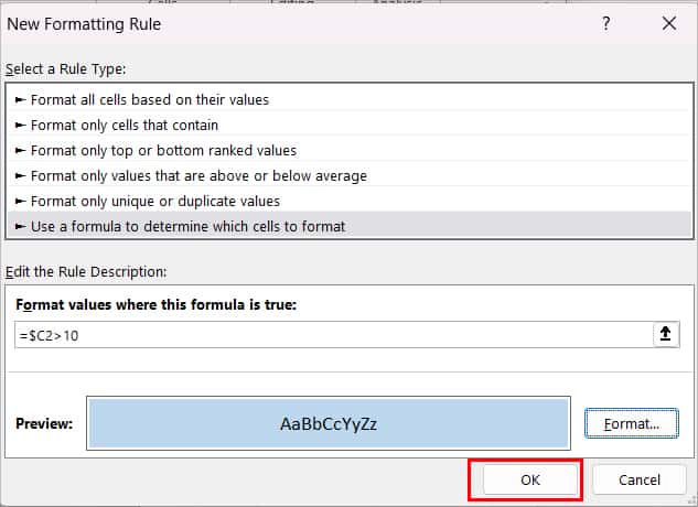
6. Again, click on OK button. 
   

How to Automatically Highlight Every Other Row When You Add Data in Excel?

Sometimes your data may be incomplete at the time of highlighting rows. Fortunately, there’s also a formula to automatically highlight every other row when you add new data. Let’s check them out below. 

1. Launch Excel.
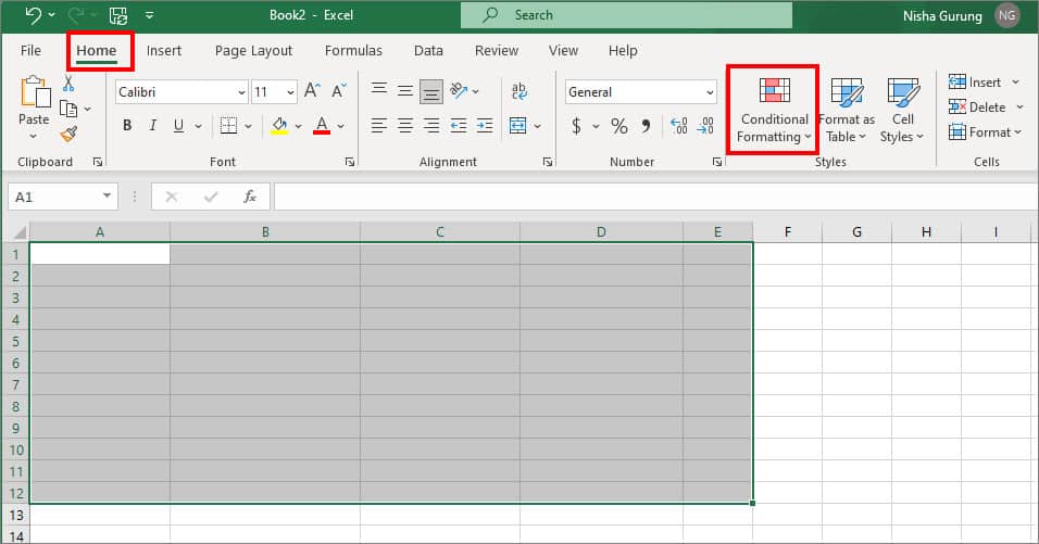
2. Open your workbook and highlight the entire Cell area. 
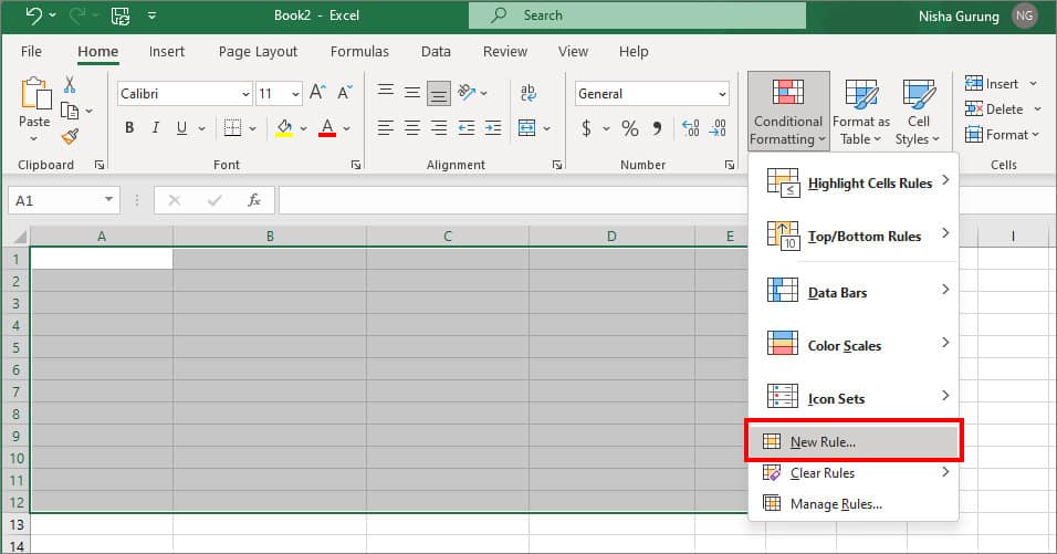
3. Click on Home > Conditional formatting.
   
4. Choose New Rule.
   
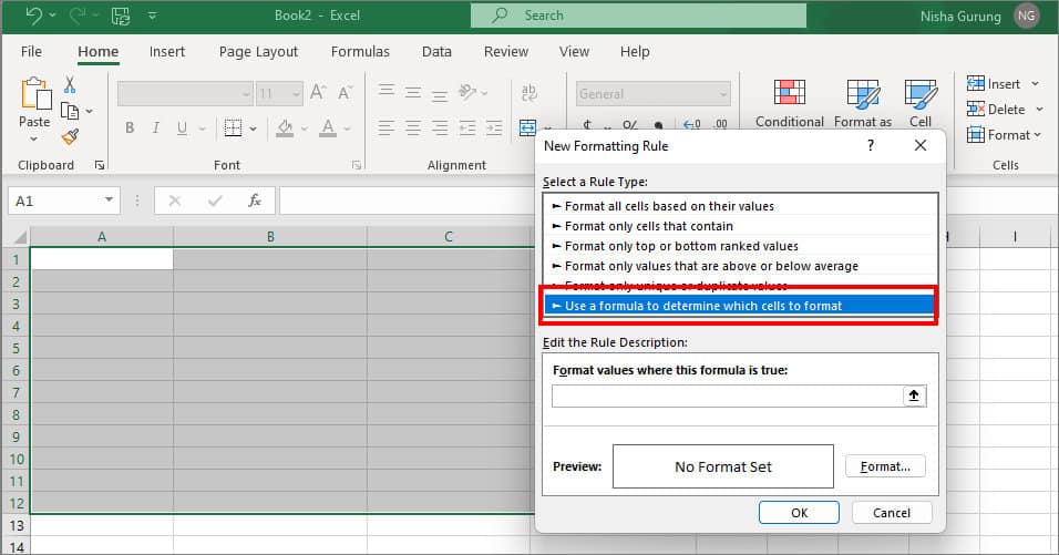
5. Under Select a Rule Type, click Use a formula to determine which cells to format. 
   
6. Enter =AND(MOD(ROW(),2)=0, A1<>””) (For A1, select the top-left cell where your data begins.)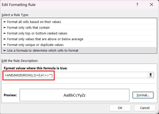
   
7. Then, choose Format.
   
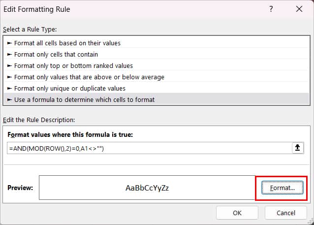
8. Click on Fill Tab. Pick a colour to highlight and choose OK.
   
9. Again, click OK.  Highlight will appear once you enter data.