In Sheets, it’s quite common to have double or triple entries on your data.
If you are in a situation where you want to identify the duplicates without removing them, highlighting values is the best bet.
Using Conditional Formatting, you can highlight the duplicate cells and make them stand out in different instances. All you need to do is create a custom formula with the COUNTIF and ARRAYFORMULA functions.
Highlight Duplicates Value in Column
Generally, we use the COUNTIF function to check and count the duplicate items in the Google Sheets. Just like that, you could enter the same formula to create a custom Conditional Formatting.
The formula will highlight the values when the COUNTIF results TRUE and won’t if it returns FALSE.
- Select the Cell Ranges.
- On Format, click on Conditional formatting. You’ll see the Conditional format rules box in the right part.
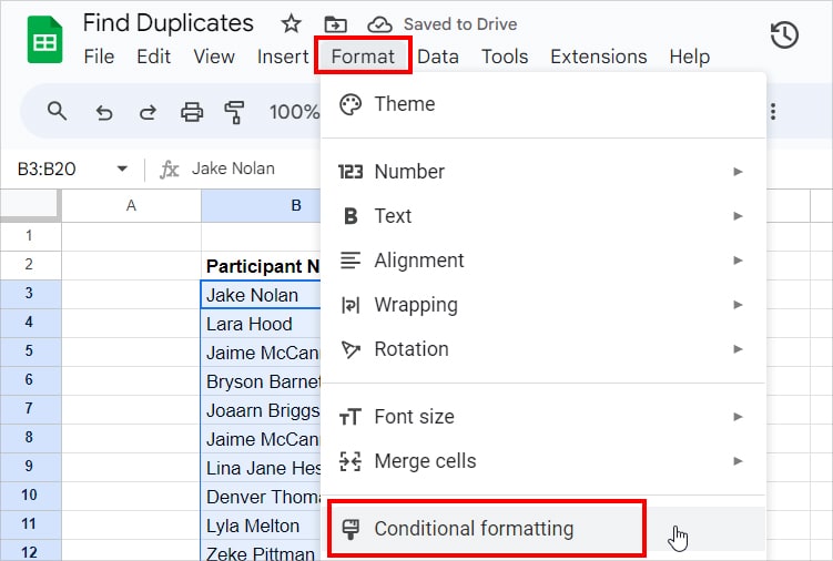
- Under Format cells if, choose Custom formula is. Then, enter any one formula.
- Highlight Duplicates in Single Column:
=COUNTIF(B:B, B3) > 1.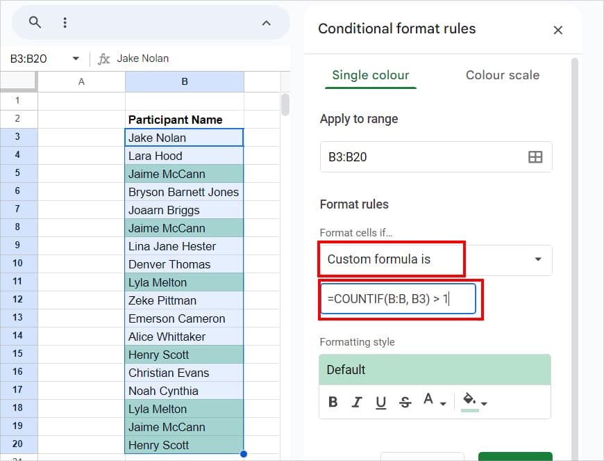
- Highlight Duplicates in Multiple Columns:
=COUNTIF($B$3:$D$10, B3) >1.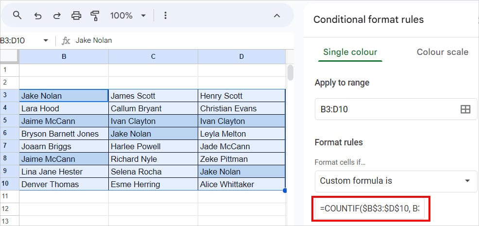
- Highlight Duplicates in Single Column:
- Below the Formatting style, expand the Fill colour and choose a Colour to Highlight. Then, hit Done.
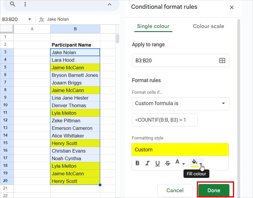
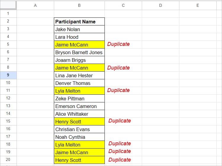
- The Formula will highlight the Duplicate Values.
Highlight Distinct Duplicates Value in Column
If you’ve noticed, the COUNTIF formula we used above highlighted all first and second duplicates.
But, assuming you only want to highlight distinct values. For example, exclude the first occurrence, “Jaime McCann” from the column and shade the other duplicate occurrences.
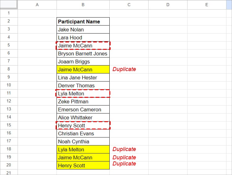
To achieve that, we can nest the COUNTIF and ARRAYFORMULA together and make criteria in Conditional Formatting.
Select your values and open the Conditional Formatting. Set the Format cells if menu to Custom formula is. Then, enter this formula
=COUNTIF(ARRAYFORMULA($B$3:$B3&$C$3:$C3&$D$3:$D3), $B3&$C3&$D3) > 1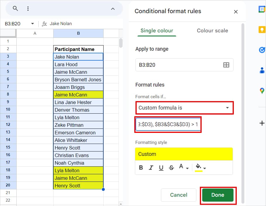
Highlight All Duplicate Rows
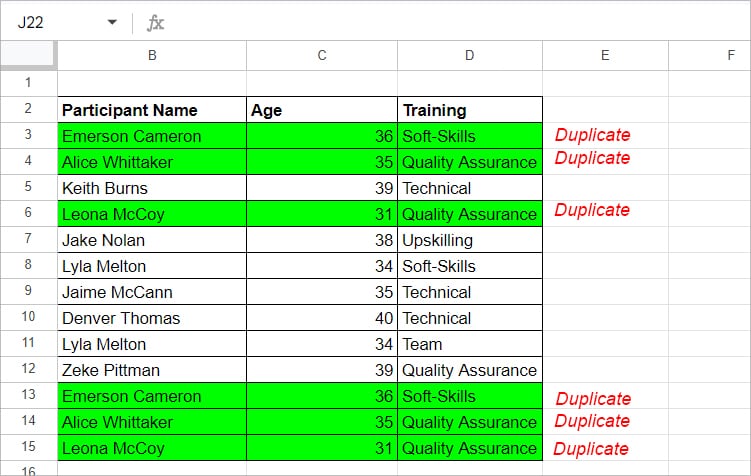
Now, let’s highlight the entire row that contains Duplicates. For that, I will use COUNTIF and ARRAYFORMULA.
Open Conditional Formatting and pick Custom formula is.
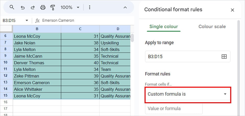
Below it, type the formula.
=COUNTIF(ARRAYFORMULA($B$3:$B$15&$C$3:$C$15&$D$3:$D$15), $B3&$C3&$D3)>1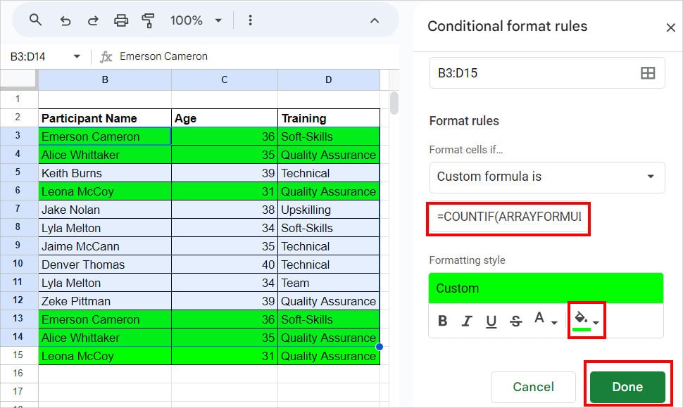
Choose a Shade in the Formatting style and click Done to highlight the row.
Highlight Duplicate Rows Based on One Column
There can be instances when you want to highlight entire duplicate rows but based on one column.
For example, here, I have the Participant’s Name, Age, and Training. Although there are duplicate items in all columns, I want to highlight the cells based on Column B(Participant’s Name) just like the given picture.
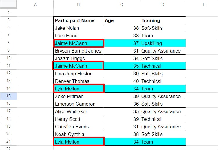
For that, first, open the Conditional Formatting menu from the Format Tab. Set Format rules to Custom formula is. Then, enter the following formula
=COUNTIF($B$6:$B$21, $B6) >1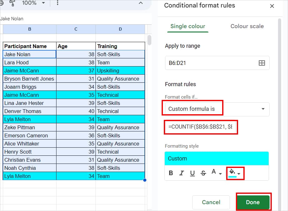
Now, on Formatting style, pick a Colour to highlight a cell and hit Done.
Highlight Duplicates Across Multiple Sheets
Suppose you want to compare the duplicate items between sheets and highlight the cell. Although you cannot directly perform that in Sheets, we have a workaround to highlight duplicate values that lie in multiple sheets.
For Example, Let me compare the Participant’s name of Sheet 1 and Sheet 3. Then, if there are duplicates, I will highlight the cells in Sheet 3.
Firstly, next to the names, I will use the COUNTIF formula to count the cells. Use the same formula as below.
=COUNTIF(A:A, A3) + COUNTIF(Sheet1!A:A, A3)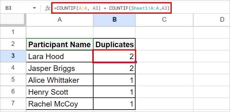
The formula returns the number of name occurrences. Here, we have 2 Names that are in both Sheet 1 and Sheet 3. Similarly, for unique names, we got 1.
Now, once we have the count of duplicate items, we can create the Conditional formatting rule and shade the cells.
Select all ranges and open the Conditional Formatting. After you choose Custom Formula is Rules, use this formula =B3 > 1. After that, select color and click Done.
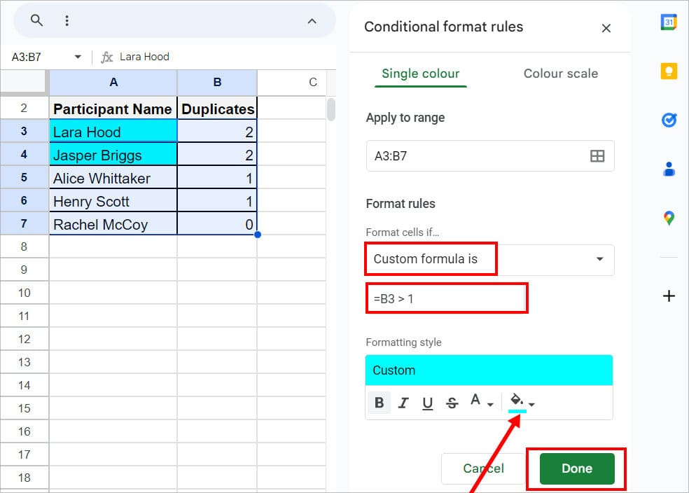
This way, the conditional formatting highlights the duplicate items based on different sheets. You can also hide the helper column if you want.