How to Use the ARRAYFORMULA on Google Sheets

In Google Sheets, the non-array functions like IF, SUM, SUMIF, MAX, AVERAGE, VLOOKUP, etc return only a single value as a result. 

But, if you want these functions to result in multiple arrays, Google Sheets has a dedicated function called ARRAYFORMULA for this purpose. 

You can nest ARRAYFORMULA with non-array functions. The function only takes one argument which is array_formula.

Syntax: 

=ARRAYFORMULA(array_formula)

Here, the argument can be cell ranges, a function returning > 1 output, or a mathematical expression of the same size.

In this article, I will cover all the examples you could use the ARRAYFORMULA. 

ARRAYFORMULA with SORT

During Calculations, you may find the need to sort the numbers in ascending or descending order. Instead of manually sorting numbers and using formulas to calculate, you can perform all of these in one go.

Example:

I need to calculate an array of profits as well as sort them in ascending order. To do that, my formula will be:

=SORT(ARRAYFORMULA(1-B3:B10/A3:A10), 1, TRUE)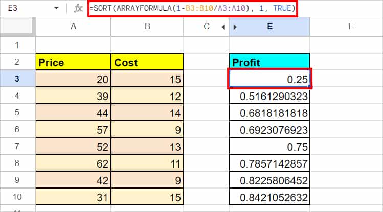

Here, the formula first calculates profit. ARRAYFORMULA returns the array of results—and finally, the SORT function reorders it. 

ARRAYFORMULA and IF

With the Google Sheet’s IF function, you can return a specific item when the Condition is met and not met.

Let’s use the ARRAYFORMULA with IF to get the multiple items for the Condition.

Example:

Suppose I need to check whether the Quantity of a Product is greater than 15 or not. Now, if I used this =IF(C6:C13 > 15, "Yes", "No") formula, I’ll get a single value and would have to copy it down for the rest of the columns.

But, If I just converted the formula into an array, it will immediately return the output for all inputs. Isn’t it so much quicker and better to perform calculations?

To do that, here’s my formula

=ARRAYFORMULA(IF(C6:C13 > 15, "Yes", "No"))

ARRAY FORMULA with SUMIF

The SUMIF function is used to add a cell range in certain criteria. But, let’s calculate the conditional sum for multiple values at once.

This method is especially useful when you have the same criteria and the same Array range.

Example:

Here, I have a column for Product, Price, and Quantity. I want to add the quantity for all of these products at once.

For that, I entered the formula as

=ARRAYFORMULA(SUMIF(A6:A, G6:G8, C6:C13))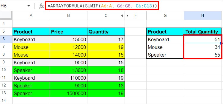

In the SUMIF, our criterion is to add the cell ranges that are the same as the Product Column. 

ARRAYFORMULA with VLOOKUP

We all know the VLOOKUP function itself can return only one item from the Lookup table.

But, if you use the ARRAYFORMULA nested, you can return multiple items just like the XLOOKUP. 

Example:

Using the VLOOKUP table, let’s return the Product ID, Stock, and Price for our Lookup Value. I entered this formula,

=ARRAYFORMULA(VLOOKUP($G$4, $A$4:$E$8, {2, 4, 5}, FALSE))

As you can see in the VLOOKUP formula, I have specified to return value from 3 columns which is enclosed inside the column brackets {2, 4, 5}. Then, the ARRAYFORMULA function returns those items.

ARRAYFORMULA with SUM and IF

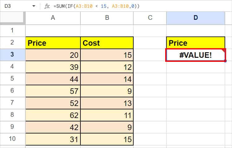
Unlike Excel, Google Sheets does not calculate the formulas with SUM and IF nested together.

For example, if you enter =SUM(IF(A3:B10 < 15, A3:B10,0)) formula, you’ll receive a #VALUE! error.

But, if you put the ARRAYFORMULA in the beginning, it’ll return the results. 

=ARRAYFORMULA(SUM(IF(A3:B10 < 15, A3:B10,0)))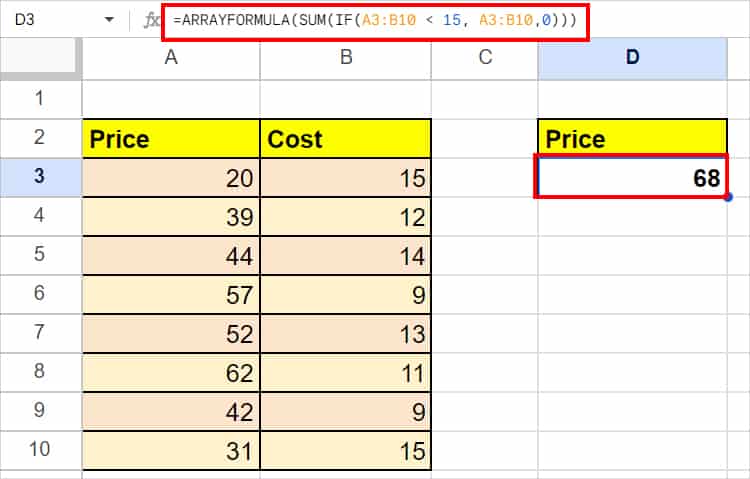

The formula resulted in 68 as output. 

ARRAYFORMULA with UNIQUE, FILTER, COUNTIF

Suppose, I want to return only the unique values from the columns that have duplicates.

For that, I can use the ARRAYFORMULA nested with UNIQUE, FILTER, and COUNTIF to easily extract the required unique values.

=FILTER(UNIQUE(C6:C13), ARRAYFORMULA(COUNTIF(C6:C13, UNIQUE(C6:C13))>1))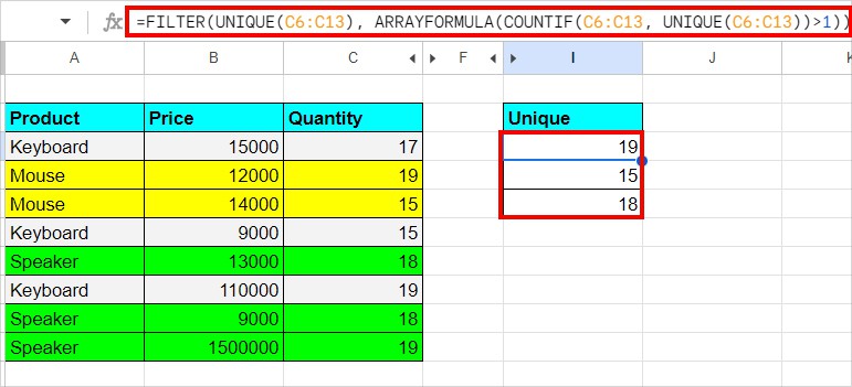

The formula resulted in 3 unique values from Column I. 

How to Use ARRAYFORMULA To Extract Data From Another Sheet?

ARRAYFORMULA is not only limited to returning an array of results. You can also use it to pull out data from another sheet. 

Example:

Suppose I need to extract B3:B10 range from Sheet 1. For that, my formula would be:

=ARRAYFORMULA(Sheet1!B3:B10)

Things You Should Note When Using ARRAYFORMULA

• There’s a keyboard shortcut to activate the ARRAYFORMULA. So, you wouldn’t have to enter =ARRAYFORMULA() every time. After typing the formula, press Ctrl + Shift + Enter keys instead of just Enter key. 
• A Curly Bracket { at the start of the formula also means the formula is an ARRAYFORMULA.
• Google Sheets does not allow you to export the ARRAYFORMULA. 
• To prevent the #SPILL! Behavior while using this function, make sure there’s space to return the array of results in your spreadsheet.
• Use ARRAY_CONSTRAIN Function with ARRAYFORMULA to control the unnecessary calculation of array results. 

When Not to Use ARRAYFORMULA?

Some of the Google Sheets functions like SUMIFS, IFS, and AND functions do not work with the ARRAYFORMULA.

So, if you attempt to use the ARRAYFORMULA with those functions, it’ll result in an error or no changes.