Did you just spend a whole lot of time entering a piece of information, only to realize you no longer need the data? Unfortunately, we cannot bring you back the time you spent entering the data but, what we can do is help you save time in deleting them.
Excel has three features – Find & Select, Sort & Filter, and the Find & Replace command that will help you in the process of locating and deleting values. You can use these tools to first select the data, and then use Ctrl + – to delete them. If you’re not a big fan of shortcuts, you can use the Delete option in the Home ribbon to delete the selected values.
Find & Select
The Find & Select tool comes in handy when you’re looking for more than just data on your spreadsheet. The utility helps you select almost everything including formulas, comments, conditional formatting, constant values, data validation, and objects.
- Open your worksheet.
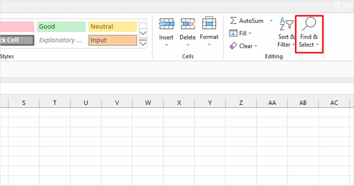
- On the Home tab, select Find & Select.
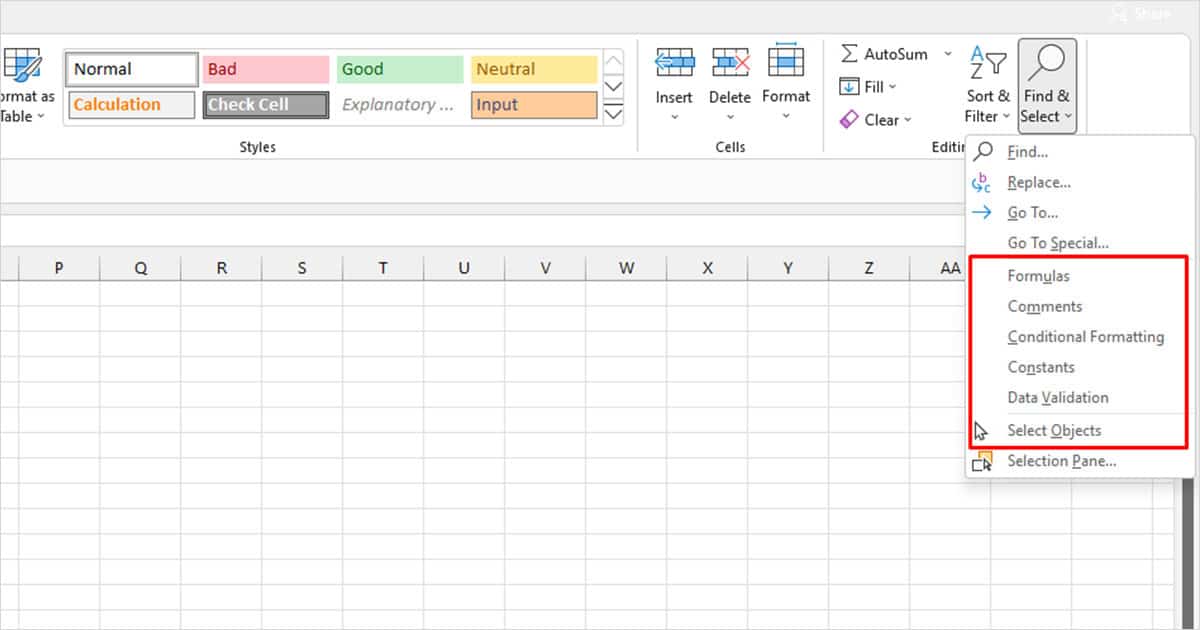
- From the drop-down, select one of these:
- Formulas: To select cells with formulas.
- Comments: Selects cells with embedded comments.
- Conditional Formatting: To select cells with conditional formatting rules.
- Constant: Selects cells with static values.
- Data Validation: To select cells with data validation.
- Select Objects: Selects objects in your sheet.
On your keyboard, select Ctrl + – to delete the selected cells.
Sort & Filter
Sort and Filter is the perfect tool if you’ve entered your data under a table. Even if you haven’t inserted a table, you can still use the tool if your data is under a range.
You will not have to insert Filter if your data is under the table. If your information is however in a range, select the first cell of the range and head to Home > Sort & Filter > Filter.
- Select the drop-down icon on the column header.
- Deselect the box next to Select All.
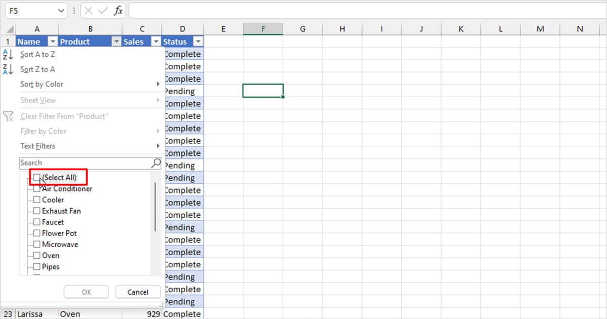
- On the search bar, type the data you wish to delete and hit Enter.
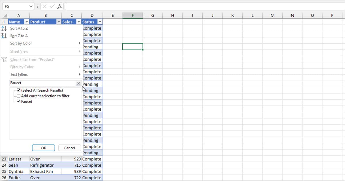
- The tool will show only the data you wish to delete. Select the data.
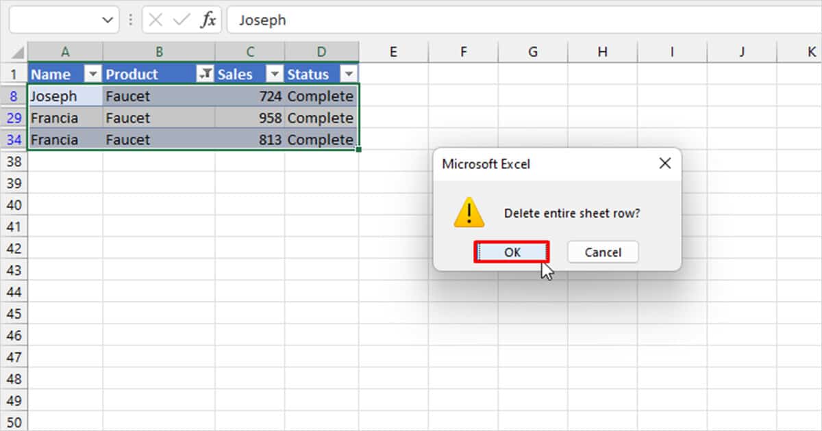
- Use Ctrl + – to delete the values.
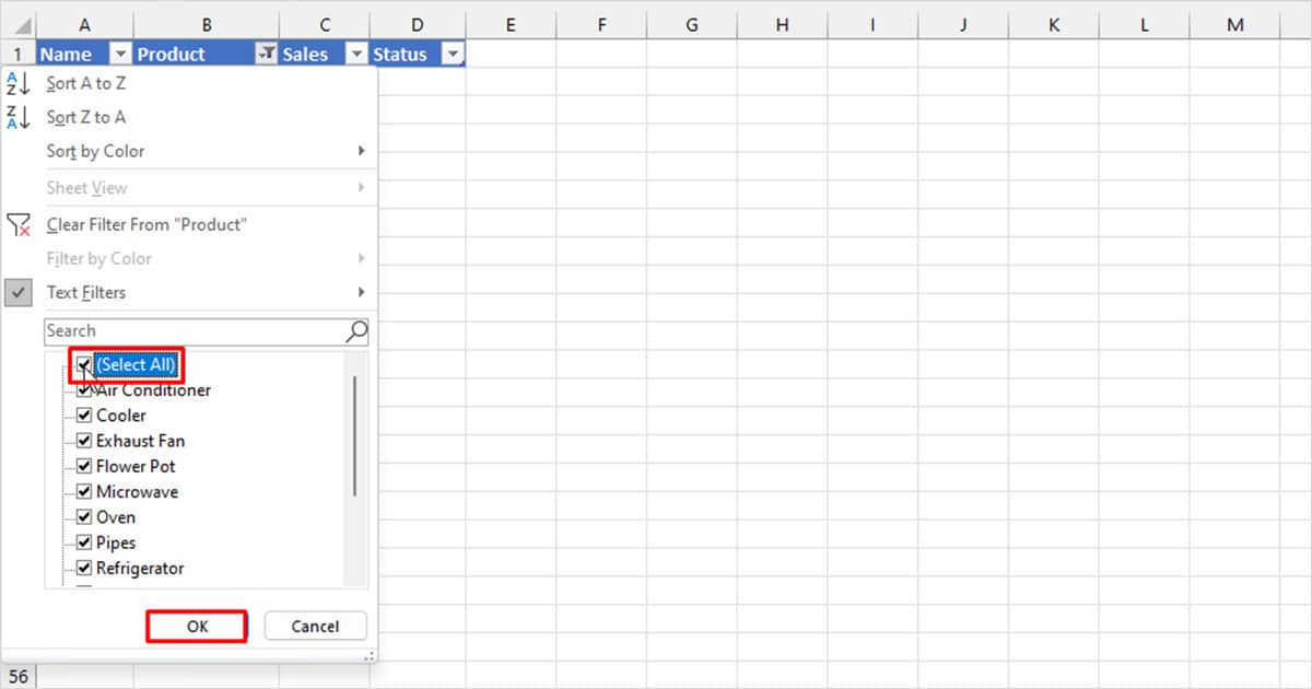
- Click on the drop-down menu again and select Select all, and hit Enter.
Find and Replace Command
You can use the Find and Replace command to not only select the cells to delete them but, you can also swap the existing value with a new value.
To better explain this utility, we have a sales sheet as an example. We’re looking to filter out all records with the “Complete” status.
- On your keyboard, hit Ctrl + H.
- Select the Options >> button.
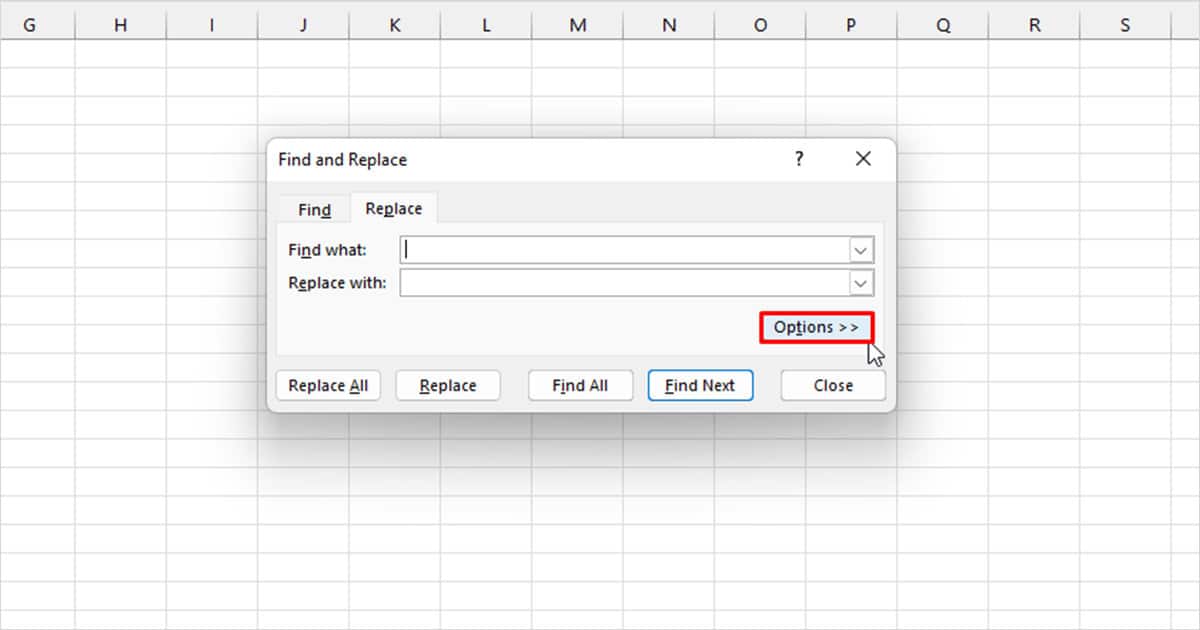
- Next to Find what, we entered Complete.
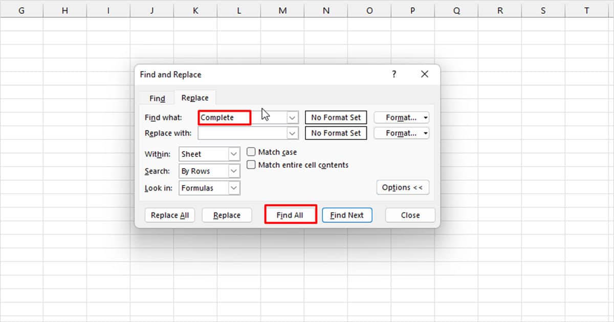
- Leave the Replace with section empty. (If we were looking to swap “Completed” with another value, we’d enter our replacement value in this section and then click Replace All.)
- Click Find All.
- The tool will display all the cell items with the value in a pop-up below the window. Select the first item and scroll down to the last item.
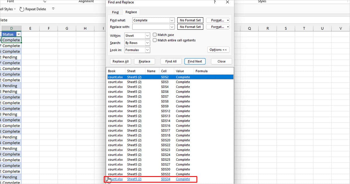
- Hold down the Shift key and click on the last item.
- Close the Find and Replace Window.
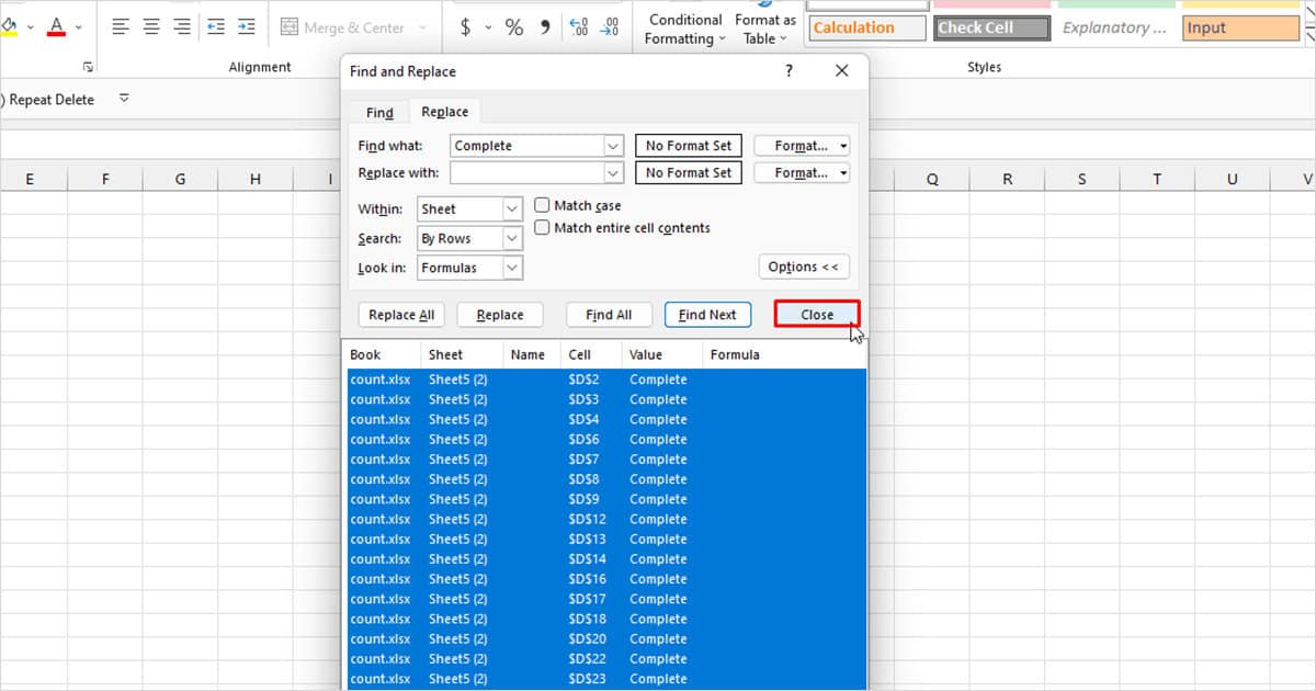
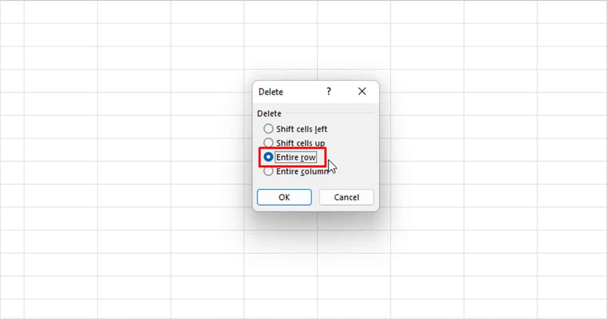
- On your keyboard, use Ctrl + –.
- Select Entire row > OK on the pop-up.
Related Questions
How to Find Duplicate Values
You can use conditional formatting to locate duplicate cells in your Excel grid.
- Select your range from the grid.
- From the Home tab, select Conditional Formatting.
- Choose Highlight Cells Rule > Duplicate Values.
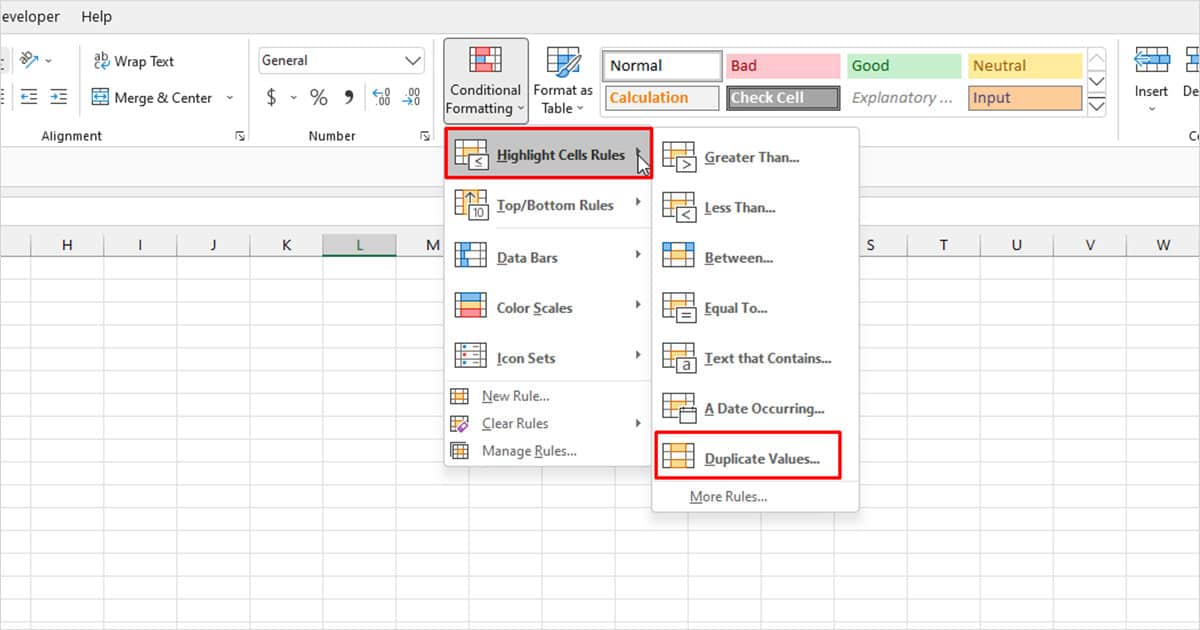
- On the pop-up, pick a format next to values with, then click OK.
How to Delete Duplicate Values
The Power Query is a powerful tool that could help you in filtering your data, including deleting empty rows and duplicate values. The simplest way to find and delete duplicate values is by using Power Query. However, Power Query is case-sensitive, meaning that it will not delete the same values in different cases (like Apple and apple).
- Select your range from your worksheet.
- Head to the Data tab and select From table in the Get & Transform section.
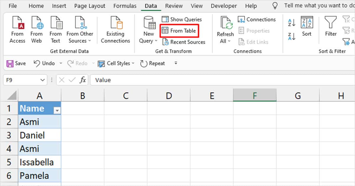
- If you see the Create Table pop-up, click OK.
- Right-click on the column header and choose Remove Duplicates.
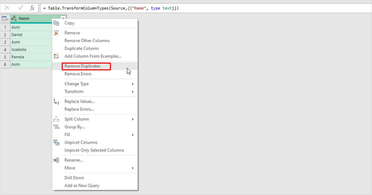
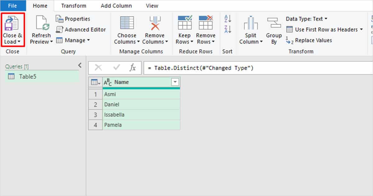
- From the Home tab, click Close & Load.
