Excel allows you to create a different line on the same cell using the Excel shortcut, Alt + Enter. Many users prefer breaking lines to fit multiple characters in the same cell without stretching the cell horizontally.
However, if you change your mind about the line breaks, you may realize that compiling them together in one line is tedious. Fortunately, you can use some of Excel’s tools and features to speed up the process.
Clear Format
Line Breaks are simply a format. If you clear the formatting you’ve applied to the cells, Excel will put your data in the same line again. However, do not use this method if you have other formatting applied to your cells because Excel will all formatting from the select cells.
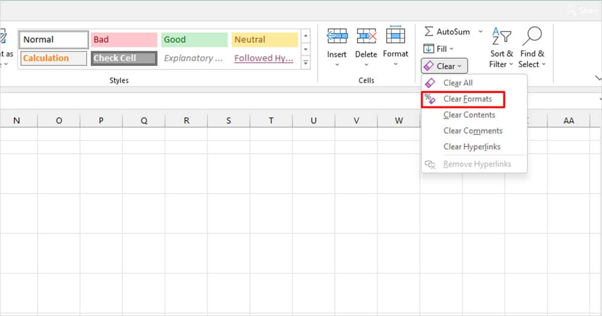
- Head to the Home tab.
- Select Clear from the Editing section.
- Choose Clear Formats.
Refer Cell with Line Breaks on a Different Cell
If you’ve used a delimiter, like space, after each element, you can simply use cell referencing. You can also use this method if you do not have a delimiter, however, know that when you compile your data in a single line there will be no symbol separating it.
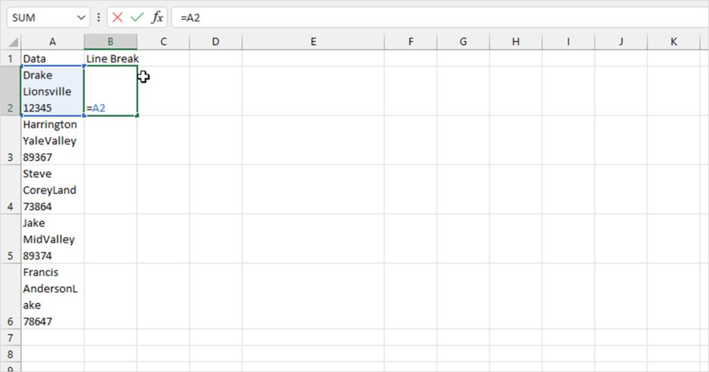
For example, cell A2 has about three line breaks. Each element has space in between them. In a different column, we simply entered =A2. This gives us the data in cell A2 without the line breaks. You can then drag the fill handle to convert the remaining values.
This is because line breaks are a formatting feature. When Excel uses cell referencing, it only references the data and not the format. If you’re looking to delete the original source, WAIT! The reference is still dependent on the cells with the line breaks.
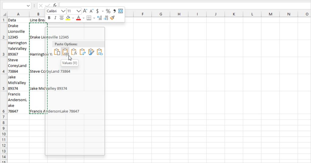
What you can do as a workaround is paste only Values from the Paste Options. Copy the values from the destination cell range and right-click on it. Use the V key on your keyboard and there you have it! Excel will only paste only the values, without the formula. You can then clear the original source without data in the destination range getting cleared out.
Use the Find Command
The Find Command is one of the fastest ways you can remove line breaks from your entire worksheet. The only downside to this method is that it lacks customizability and you do not have the option to remove line breaks in specific cells as it applies to the entire grid.
- On your keyboard, use Ctrl + H.
- Next to Find what, use the combination Ctrl + J. You might see a small dot of nothing at all.
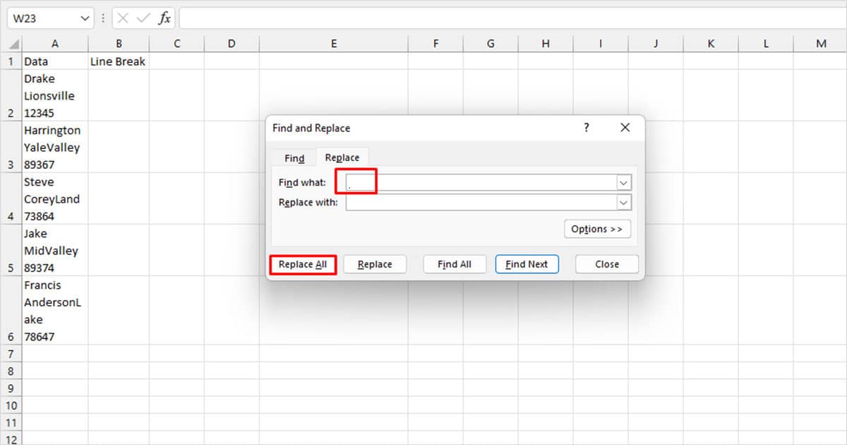
- Depending on if you want to add a delimiter, enter a symbol next to Replace with or leave it empty.
- Click Replace All.
Use the SUBSTITUTE Function
Before we move on to explain this method, let’s learn a bit about ASCII. ASCII, the abbreviation for the American Standard Code for Information Interchange assigns a number for each special character, including Line Breaks.
The ASCII number for Line Breaks is 10. We will be using this information to replace line breaks with a delimiter, or nothing if you have a delimiter in use.
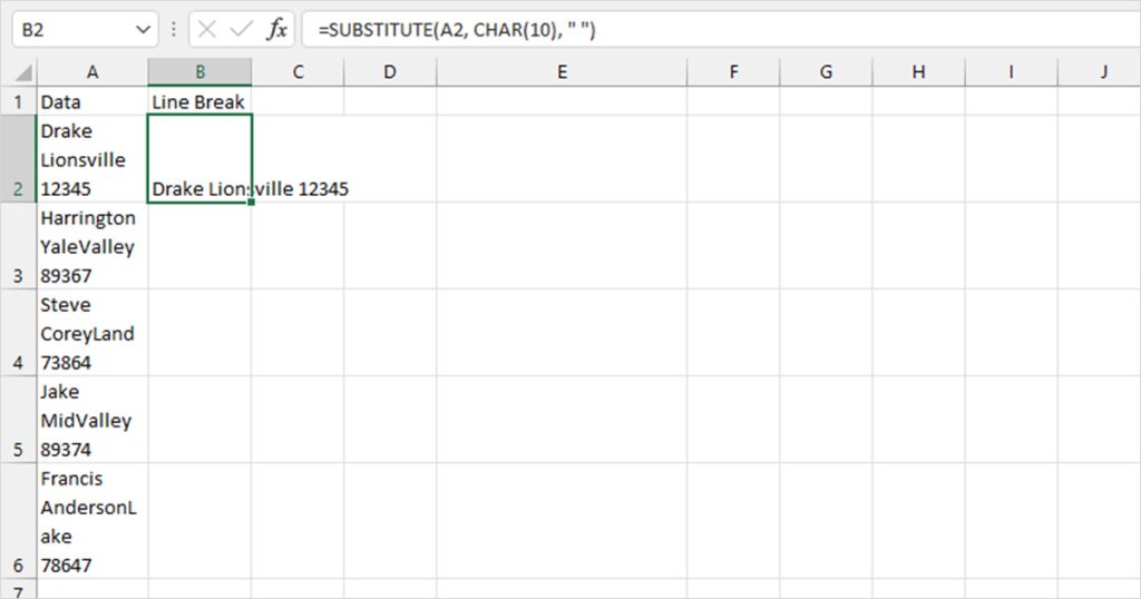
Column A has five values with line breaks. Here is the formula we used to separate these values in cases where there’s no delimiter.
=SUBSTITUTE(A2, CHAR(10), “ ”)
You can modify the formula depending on your cell value and your preferred delimiter. For example, if you do not wish to add an extra space between the values that once had line breaks, replace the third argument from “ ” with “”. Similarly, if you wish to add a comma instead of a space, use “ ,” instead of “ ” in the third argument.
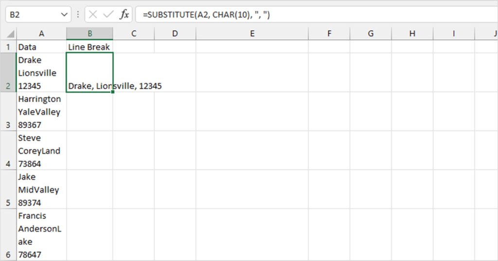
Again, with this method as well, please use Paste Options to paste values if you’re looking to delete the original source.
Clean Your Cell Using Power Query
Power Query is an excellent automation tool that will get your work done swiftly. We however only recommend this step if you have entered a separator between your values, or if you prefer to assemble the data without a divider.
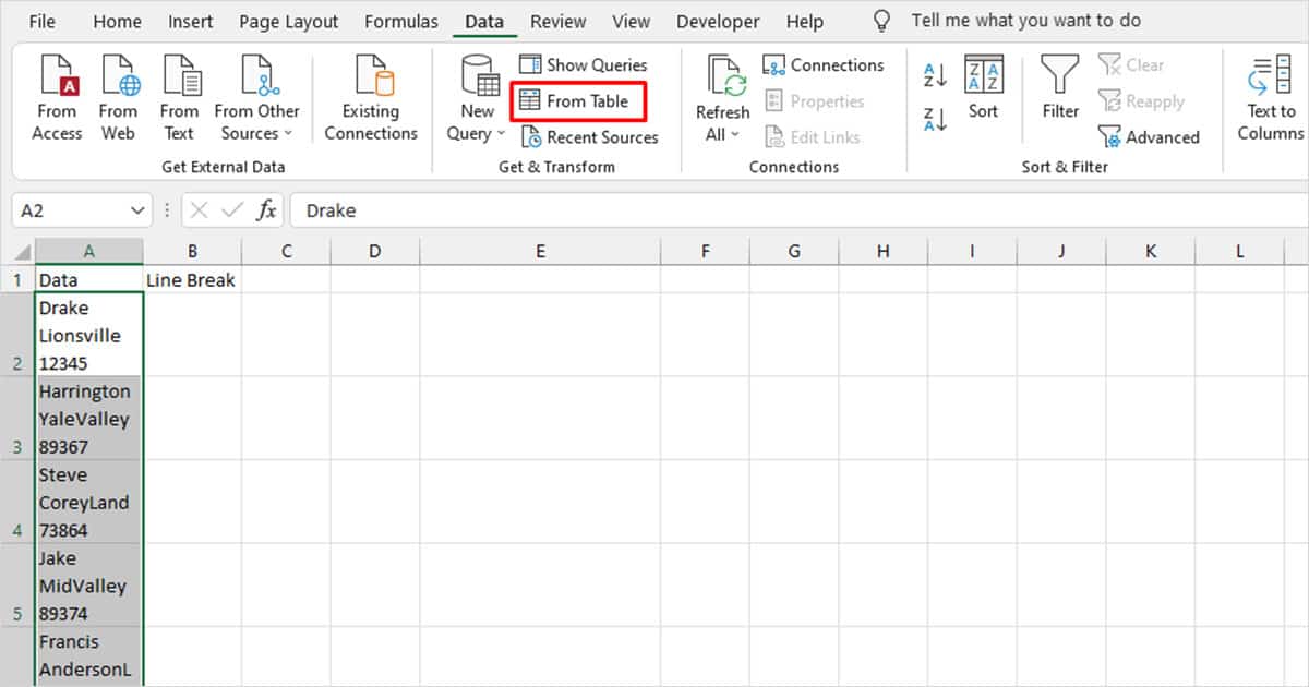
- Open your worksheet and head to the Data tab.
- Select From Table in the Get & Transform section.
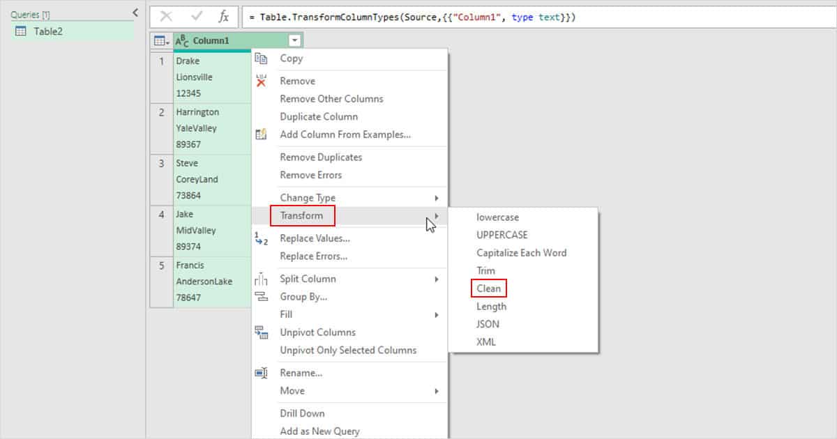
- In the Power Query editor, right-click on your column and choose Transform > Clean.
- Close and Load your data from the Home tab.
Create a Custom Function
Let’s make removing line breaks easier; let’s create our own function! Excel uses VBA to create functions and macros. You will first have to enable the Developer tab from File > Options > Customize ribbon.
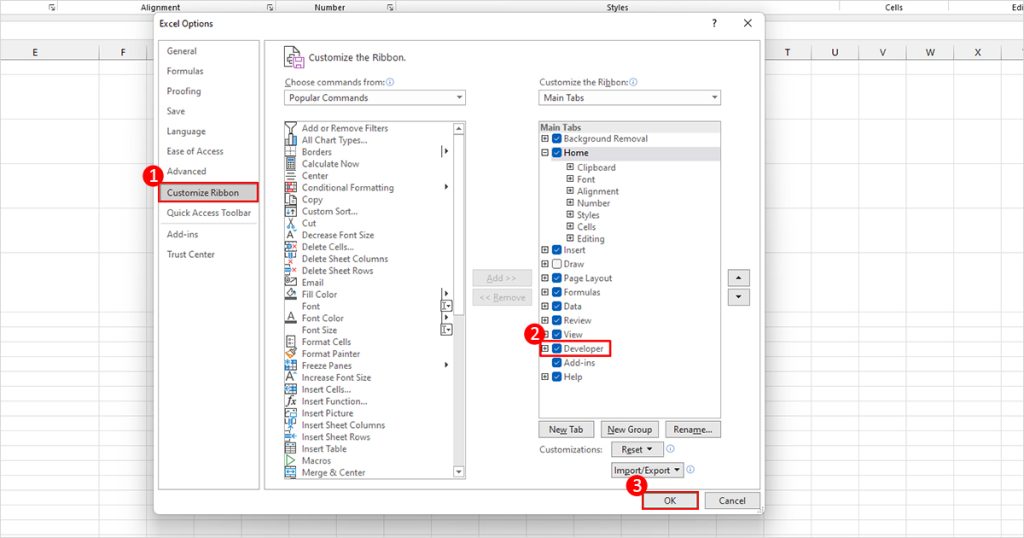
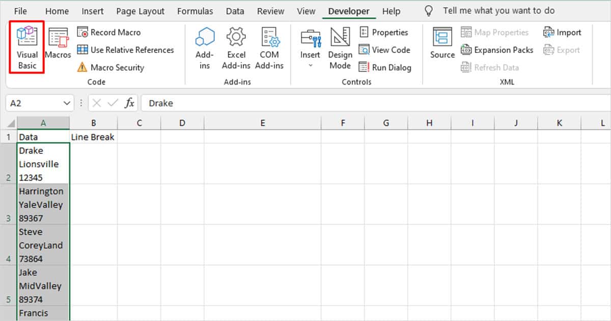
After you enable the Developer tab, you can access the Visual Basic option to create your own function.
- Head to the Developer tab and select Visual Basic.
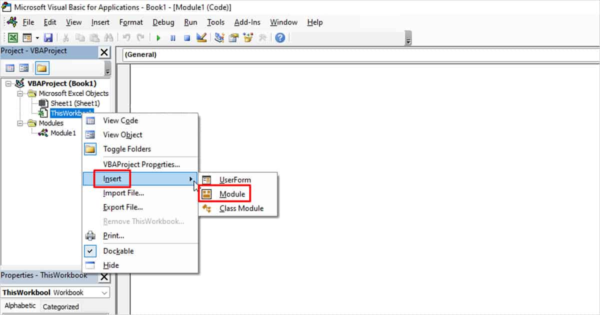
- Right-click on your sheet from the sidebar and select Insert > Module.
- Enter the following code on the window to your right:
Function RBreaklines(cell As String) As String
Dim Result As String
Dim count As Integer
Let celllength = Len(cell)
For count = 1 To celllength
If Mid(cell, count, 1) = Chr(10) Then
cell = Replace(cell, Chr(10), ", ")
End If
Next
RBreaklines = cell
End Function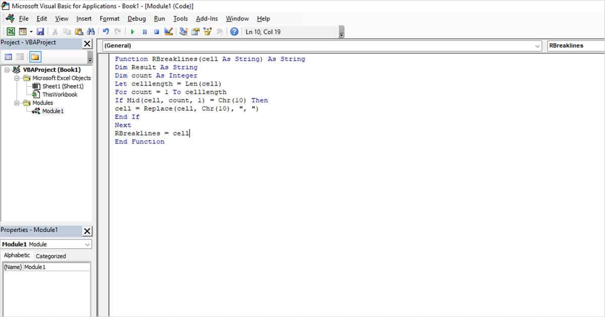
You can then use the function like you would use any other function. As an argument, pass the cell you wish to remove line breaks from and you’re good to go. Here is how your data will look after you pass it using the function.