By default, the gridlines in Excel don’t appear while printing. This is because gridlines exist in Excel only as a way to separate cells within the program. However, you can tweak a few settings to make the gridlines visible when printing out your spreadsheet.
With that said, even if you’ve enabled gridlines, there are a few nuances that can hide gridlines when printing. We will first look into the steps to print gridlines in Excel, then go into other factors that may put a hard stop to this process.
How to Enable Gridlines for Printing in Excel
Your gridlines will not print unless you enable this option in Excel. Before you look into other fixes, make sure that this setting is configured for your worksheet.
Remember, you must enable this setting every time you want to print gridlines. So, if you have multiple spreadsheets you want to print gridlines for, hold the Ctrl key and select them from the worksheet view.
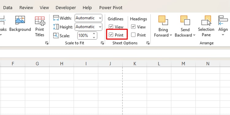
- On your worksheet, go to the Page Layout tab.
- Check the box for Print in the Sheet Options section.
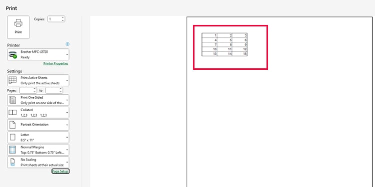
- On your keyboard, hit Ctrl + F2 to go to the Print tab.
- Check if there are gridlines around your data.
Still Can’t Print the Gridlines?
If you don’t see gridlines in the print preview even after you enable the gridlines for printing, there could be other factors behind this issue. Check if you have any of these elements on your spreadsheet:
- Shading in Cell
- Conditional Formatting
- White Borders
- White Gridline Color
These factors hide gridlines in Excel, making them invisible when printing. We will be discussing how you can disable these formattings, including an additional print configuration that hides gridlines while printing.
Remove Cell Fill
If you have filled your cell with any color, it will hide the gridlines. This is not only true for printing, but also when you’re working on your spreadsheet. If shading the cell does not add a lot of value to your data, you can remove them.
- Select the range that contains the formatting.
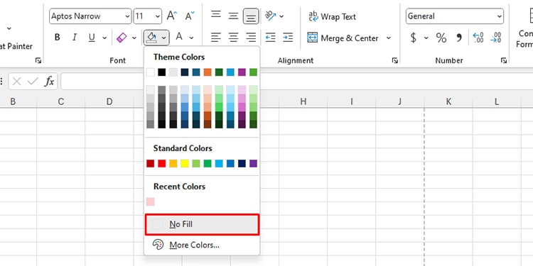
- Head to the Home tab.
- Select the fly-out next to the fill bucket.
- Choose No Fill.
Change Conditional Formatting
You can choose from a list of formats for conditional formatting. If you’ve set the condition to fill cells, it’ll have the same effect as manually shading your cell; it will hide the gridlines.
Instead of setting the formatting rule to fill your cell, you can change the settings to apply other formatting to the cell that meets the set condition.
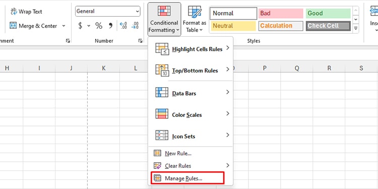
- Go to Home.
- From the Styles section, select Conditional Formatting.
- Choose Manage Rules.
- Select your Conditional Formatting rule and go to Edit Rules.
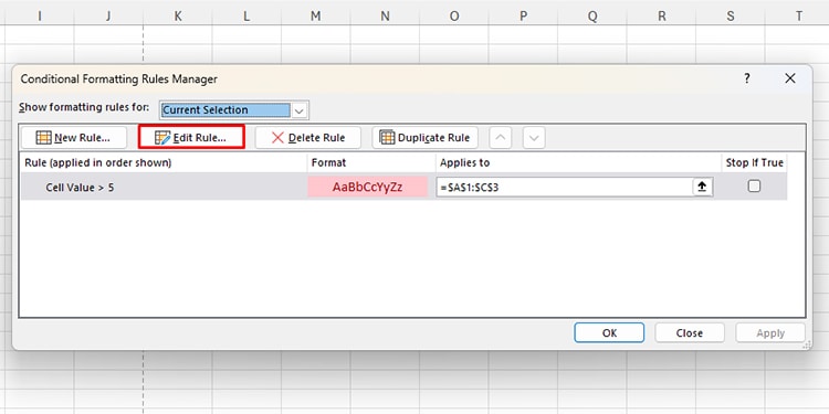
- Click on the Format button.
- Head to the Fill tab and click on Clear.
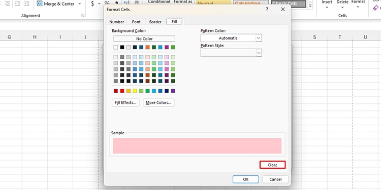
- Select OK > OK > OK.
Apply Borders
If you can’t remove the shading you applied to your cell, you can simply add borders to your range. Make sure that the borders are not of the same colors as the cell shading, or else they won’t appear while printing.
- Select the range you wish to apply borders to.
- Go to the Home tab.
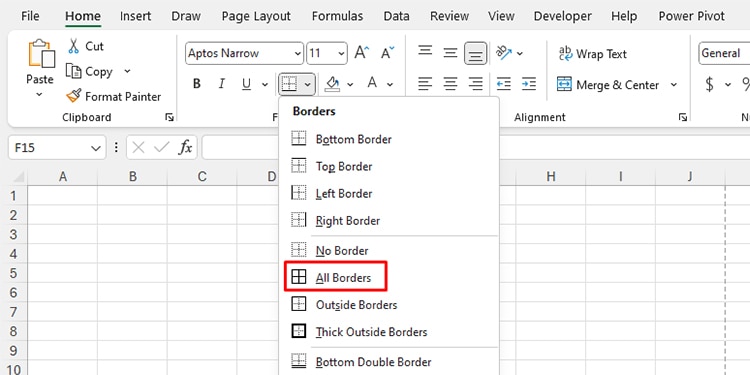
- Click on the fly-out menu next to Borders in the Font section.
- Select All Borders.
Change the Border Color
If you still can’t see gridlines after you’ve applied borders, you must’ve chosen the wrong color. You will not see your borders if they clash with the background color. The background color could be either the cell shading or the default background color – white.
If you haven’t applied any shading, make sure your borders aren’t white. Similarly, if you’ve filled your cell with color, make sure your border isn’t the same color as that.
- Go to Home and select the fly-out next to the border icon.
- Select Line Color then choose a color.
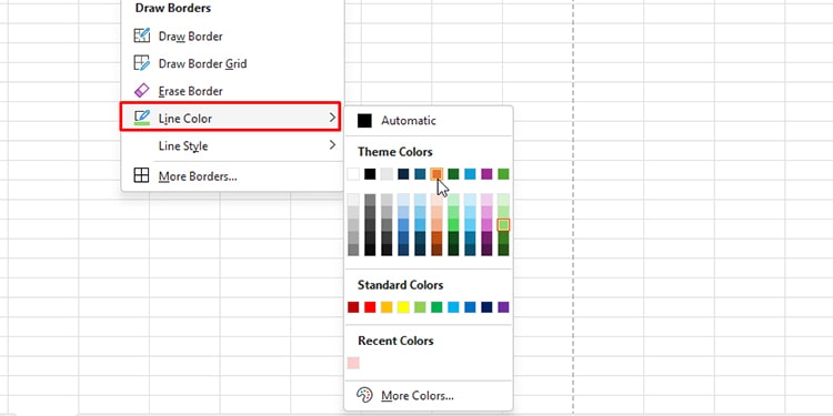
- Select your range, and click on fly-out next to the border icon.
- Choose All Borders.
Change the Gridline Color
If you’re into personalizing your Excel space, you could’ve mistakenly changed the color of your gridline to white. As the background color of the Excel spreadsheet is white, white gridlines will most certainly disappear from sight.
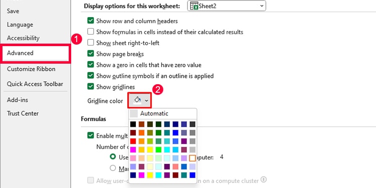
If you think this could be the reason, you can change the color of your gridlines from Excel Options. You can choose from a number of theme colors, for your gridlines in Excel.
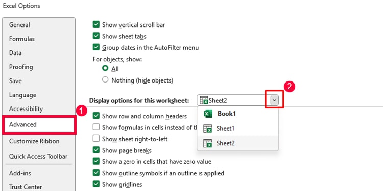
- Head to File > Options.
- Go to Advanced.
- Next to Display options for this worksheet, choose your worksheet.
- Under the same section, choose a color next to the Gridline color.
- Click OK.
Disable Draft Quality
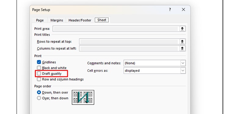
While trying to print gridlines on your spreadsheet, you must always make sure that the Draft Quality option is left unchecked. Draft quality refers to a test print, which lowers the quality of your document, hiding gridlines in the process.
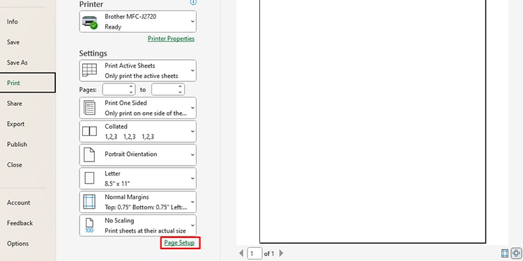
- On your active sheet, use Ctrl + F2.
- Click on Page Setup.
- Head to the Sheets tab.
- Uncheck the option next to Draft Quality.
- Click OK.