When used correctly, images in Excel can add a lot of value to an otherwise boring spreadsheet. Including an image in documents such as inventory reports, food menus, country flag lists, and so on can make them more engaging and informative.
Adding pictures to your Excel spreadsheet is easy. But, putting the image into the cell is quite tricky. The original size of the picture is floating all over the sheets. And you’ll have to realign them frequently to fit row/column sizes, which is quite annoying.
As a workaround, you can use Excel’s IMAGE Function to place pictures into cells. However, if you do not have this function, you could format images to move and size with cells or use VBA code.
Using IMAGE Function
If you want to embed an image directly into the cell, use the IMAGE Function. Yes, as surprising as it may sound, Excel has an IMAGE function specially built for this purpose.
Using this function, you can add online pictures in the supported format to your cell. It even allows you to filter, resize, use pictures in tables, etc.
But, this function is available in only Office 365 or the web versions. Your device must also meet certain system criteria to use this function. You can check them on the official Microsoft webpage.
If you can access this function, let’s get right into its syntax.
Syntax: IMAGE(Source, [alt_text], [sizing], [height], [width])IMAGE function takes up the following arguments.
- Source: Image URL link (Required)
- alt_text: Image description (Optional)
- sizing: Image dimensions to fit them in the cell.
- 0: Retains the aspect ratio of an image and fits them into a cell.
- 1: Overlooks the image’s aspect ratio and fills the cell with an image.
- 2: Keeps image in the original size.
- 3: Modify image size by entering custom height and width.
- height: Custom image height (Required when you enter 3 sizing)
- width: Custom image width (Required when you enter 3 sizing)
Let’s assume, we need to insert the image of a Pizza in the cell. For this, enter the given formula in an empty cell:
=IMAGE("https://img.freepik.com/free-photo/hawaiian-pizza_74190-2500.jpg?w=900&t=st=1679474797~exp=1679475397~hmac=498ec0210b755bddcbbd0ca86eb02de9637307276edf2df8741a1071c2f059d9", "Pizza", 1)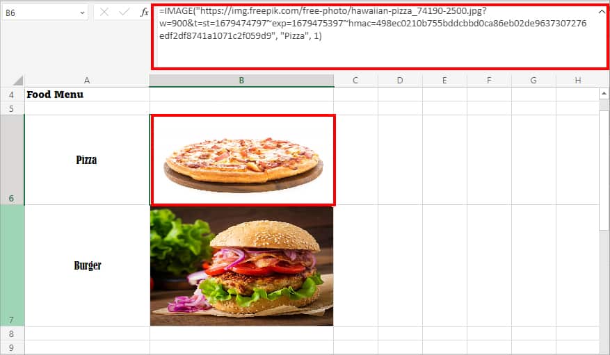
In the above formula, we have added a URL link, alt_text, and size 1 for a picture. As per size 1, it will fill the cell with images. You can also resize the picture using the row and column resize cursor.
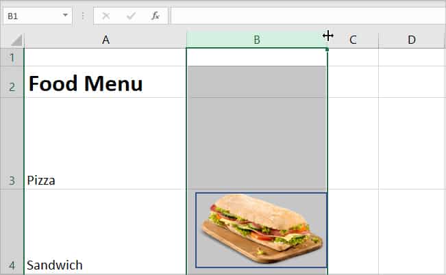
Format Image to Move and Size With Cells
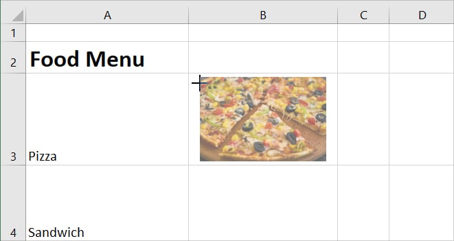
If you do not have an IMAGE function on your spreadsheet, you can add pictures as you would from the Insert Tab. Then, format the picture to Move and size with cells. By doing so, when you adjust the cell size, it will change the image dimensions too. This method is also effective for users who want to upload local pictures from the PC.
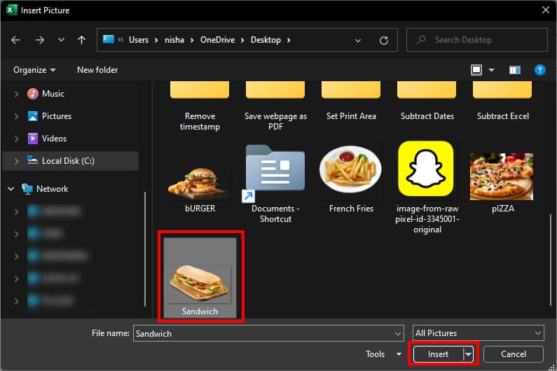
- On your Excel worksheet, adjust the row and column size as per the image.
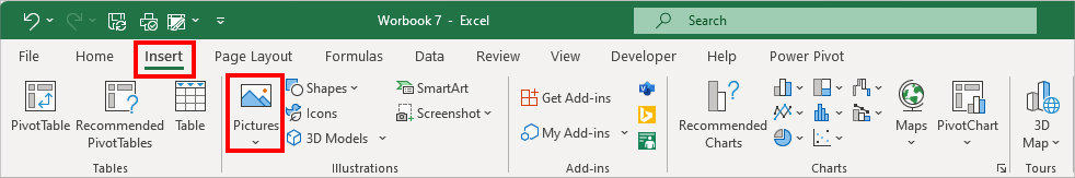
- From the Insert tab, click Pictures.
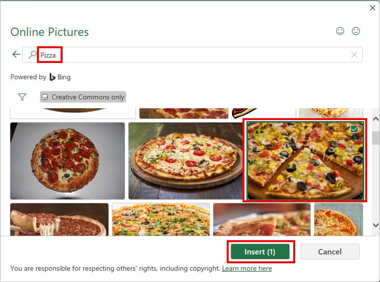
- On Insert Picture From, pick any one import location. Here, I chose Online Pictures.
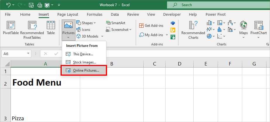
- Enter the image name in the Search bar. Select any Image and click Insert.
- Now, while holding down the Alt key, resize the image to fit the cell.
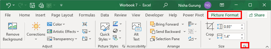
- Select the Picture and navigate to the Picture Format tab at the top. On the Size group, click on More icon.
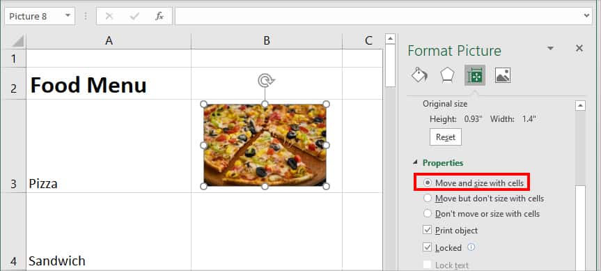
- Under Properties, pick Move and size with cells option.
From Shapes
With the above method, resizing large images to fit cell size can take a lot of time. To escape this tedious process, you can form a shape with an exact cell size and fill in the shape with a picture. When you do this, the image will also adjust its dimensions according to the cell width or height.
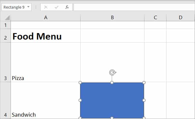
- On your spreadsheet, resize the row and column to fit the image.
- Head to Insert Tab. From the Illustrations group, click on Shapes and pick Rectangle.
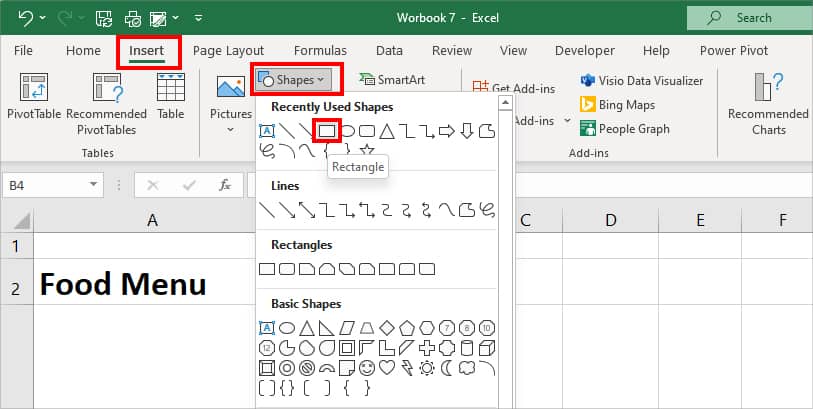
- Draw a Rectangle shape according to the column size.
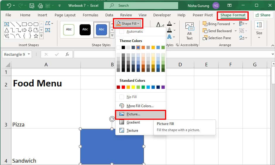
- On Shape Format Tab, click on Shape Fill > Picture.
- On Insert Pictures window, choose an option to import an image from. I picked From a File.
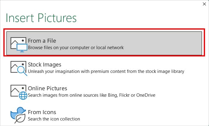
- Locate and select Image on your PC. Then, hit Insert.
- Use resize cursor to adjust images if needed.
Using VBA Code
If you get familiar with the Visual Basics for Applications (VBA) tool, it can be your favorite as it simplifies any Excel work. You just need to insert and run the mentioned code. Below, we have provided the code to resize the selected picture according to the cell grid.
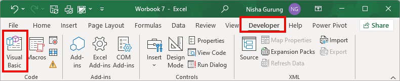
Before you begin, check if you can see the Developer Tab. If not, insert Developer Tab first to access the Visual Basic tool.
- From the Insert Tab, add an Image to your worksheet.
- Select the Image. Then, go to Developer Tab > Visual Basic.
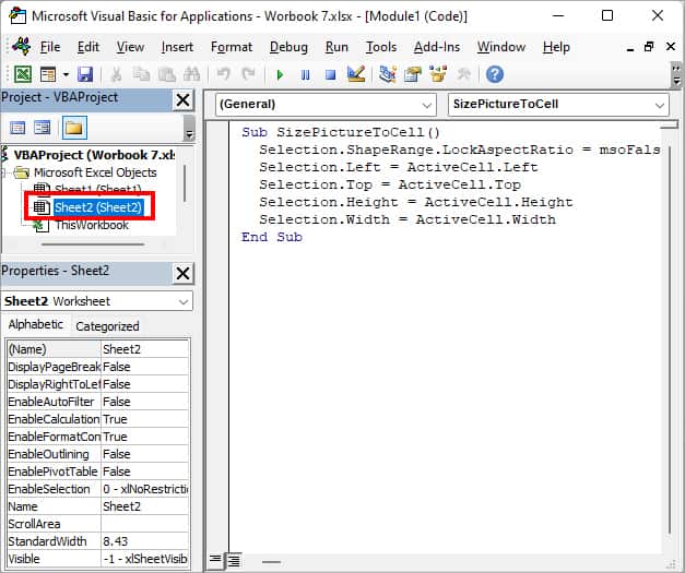
- Microsoft Visual Basic for Applications window will appear on the screen. Click Insert > Module.
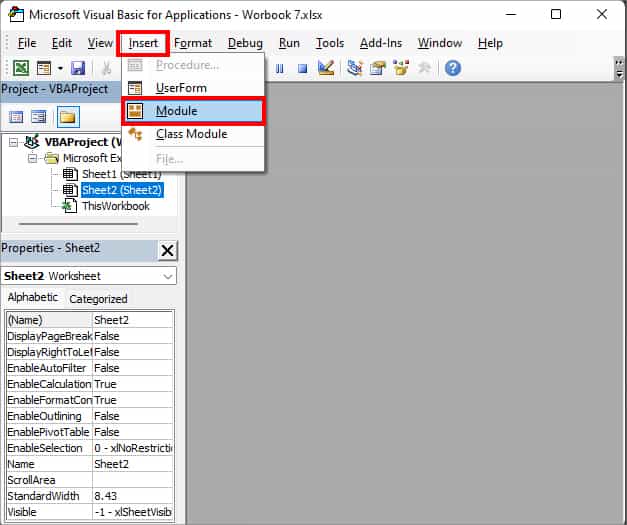
- On the blank space, paste this code.
Sub SizePictureToCell()
  Selection.ShapeRange.LockAspectRatio = msoFalse
  Selection.Left = ActiveCell.Left
  Selection.Top = ActiveCell.Top
  Selection.Height = ActiveCell.Height
  Selection.Width = ActiveCell.Width
End Sub
- Below Microsoft Excel Objects, ensure you’ve selected the correct sheet. Enter F5 to run the code.