How to Highlight Active Rows in Excel

In Excel, a green border around the cells means it is an Active cell. But, sometimes, we may struggle to see these Active Cells when the spreadsheet is excessively huge and presented on bigger screens. I know, it can be eye-straining having to skim data through endless rows and columns. 

As a primary workaround, you could use Shift + Space shortcut to select the entire row for reading the information in one view. 

But, if you have to input the value on the active cell, apply highlights with contrasting colors to make them stand out in the sheet. Here, we will learn how to shade only active rows such that you’ll automatically get highlights in any cell you select. 

Use Conditional Formatting

Most Excel users are quite familiar with Excel’s conditional formatting. This particular tool is specifically dedicated to visually shade data based on a condition. For Instance, highlight every other row, every nth row, or every active row. You can even create a rule of your own to determine the way you want to apply highlights. 

If you’re new to Excel, using Conditional formatting to highlight the active rows is possibly the most simple approach. Here, we’ve made it even easier for you as you just need to paste the formula we created.

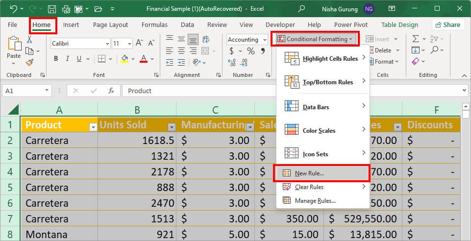
1. Press Ctrl + A to select the entire cells of the worksheet.
2. From the Home Tab, click on Conditional Formatting > New Rule.
   
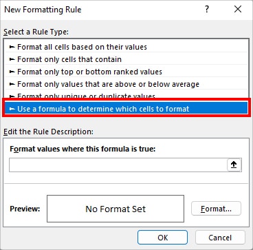
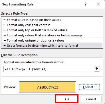
3. Under Select a Rule Type, pick Use a formula to determine which cells to format option.
   
4. Now, on Format values where this formula is true: field, paste or type in the following rule

=CELL(“row”)=CELL(“row”,A1)

5. Click Format.
   
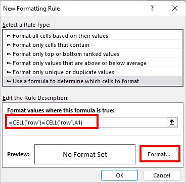
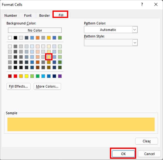
6. On Format cells, head to Fill tab and pick a color to highlight the row with. Then, click OK. 
   
7. Again, click OK.
   
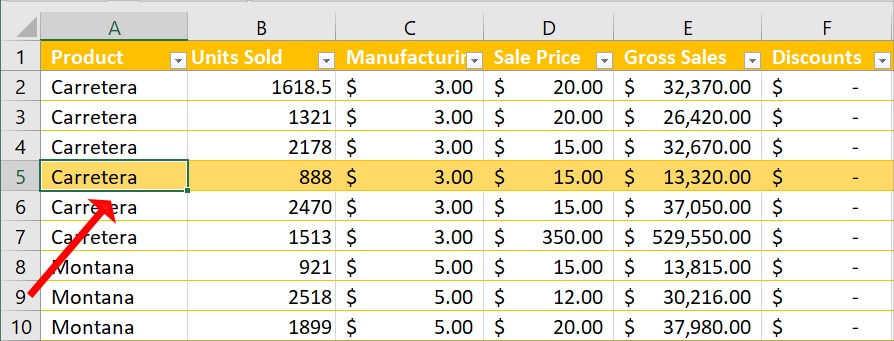
8. Now, click on any Cell and press F9 key. It will highlight the entire active row. 
   

Using Visual Basics Tool

Without a doubt, Conditional Formatting does pretty good work to shade the entire active rows. But, it still plays a partial role as you’ve to keep refreshing it.

I know having to activate your spreadsheet each time to get highlights can be quite annoying. Especially, when you’re in the midway of entering a formula in the cell as you would encounter errors like #NAME or VALUE.

But, with the Visual Basics Tool, shading only active rows is quite effective. Each time you click on the cell, it will instantly highlight all rows of active cells. The best part is, you’ve to set this format only once by pasting the code we’ve mentioned below.

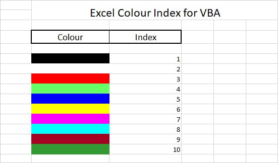
As a reference, we’ve applied a yellow color highlight for the cell by entering the 6-color index in the given formula. But, you can replace the color number with the shade you prefer to use. Before jumping into the steps, check out the color index chart in the given image. 

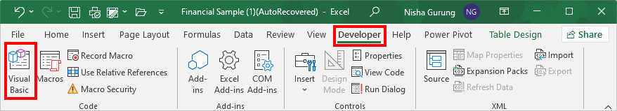
1. On your worksheet, go to Developer Tab and click on Visual Basic.
   
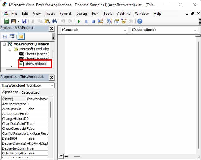
2. Under Microsoft Excel Objects, double-click on ThisWorkbook. 
   
3. Paste the given code in the empty space. 
   

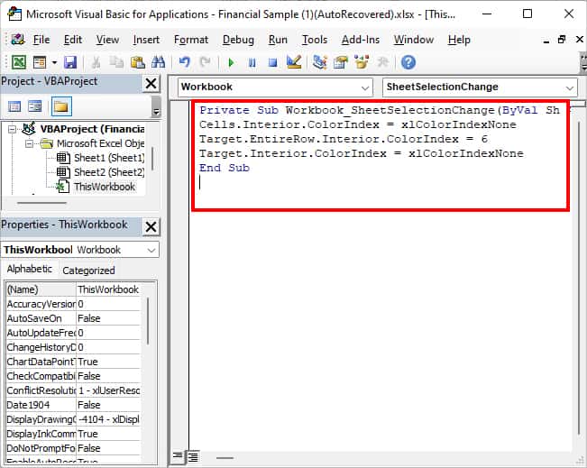
Private Sub Workbook_SheetSelectionChange(ByVal Sh As Object, ByVal Target As Range)
Cells.Interior.ColorIndex = xlColorIndexNone
Target.EntireRow.Interior.ColorIndex = 6
Target.Interior.ColorIndex = xlColorIndexNone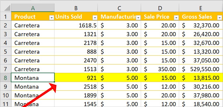
End Sub

4. Close the VBA window. On your worksheet, when you click on a cell, it will highlight the entire row of active cells.
   

How to Highlight the Active Column in Excel?

Similar to highlighting active rows, I prefer using VBA for active columns too. With this approach, whenever I click on any cell, I will immediately get highlights in the entire column.

Before starting, check if there’s a Developer tab on your sheet. For users who cannot find it, add the Developer tab first to use the Visual Basics. 

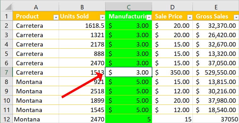
In the given steps, we will be highlighting the active color with the green color. For this, we’ve entered 4 color index in the formula. However, you can replace the number with the shade you’d like to have. See the color index chart above. 

1. Navigate to Developer Tab > Visual Basic.
   
2. Below Microsoft Excel Objects, double-click on ThisWorkbook. 
   
3. Now, Paste the given code in the empty space. 
   

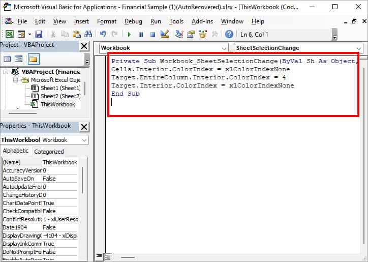
Private Sub Workbook_SheetSelectionChange(ByVal Sh As Object, ByVal Target As Range)
Cells.Interior.ColorIndex = xlColorIndexNone
Target.EntireColumn.Interior.ColorIndex = 4
Target.Interior.ColorIndex = xlColorIndexNone
End Sub

4. Close VBA window. When you select a cell, it will highlight the entire column of active cells.