Formatting is a great way you can visually separate selected cells in your spreadsheet. One of the more prominent ways to set a cell apart is by using the Fill tool to highlight certain cells.
Many users highlight the cell to color code for data analysis such as checking the status of a deal. For example, you’ve created a spreadsheet on client follow-up. The statuses are color coded as green, yellow, red, and blue implying completed, pending, declined, and non-applicable respectively.
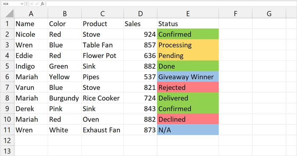
If you had a longer set of data, manually counting cells could take a village! Even unfortunate as it is, Excel has no function to assist you in this process. However, we have gathered a list of other ways you can easily count highlighted cells in Excel, so keep reading!
Find Tool
The Find tool is a lifesaver when it comes to counting cells that host a set value. However, you can also use the utility to locate cells with a selected cell format. Asides from displaying the cells with the format, you will also get the count value of the set cells.
To explain the application of this utility, we will be using the example we discussed above. We will be using the Find tool to find the number of cells with red fill.
- On your keyboard, use Ctrl + F.
- Select the Options>> button.
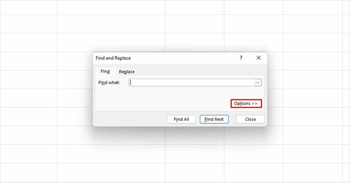
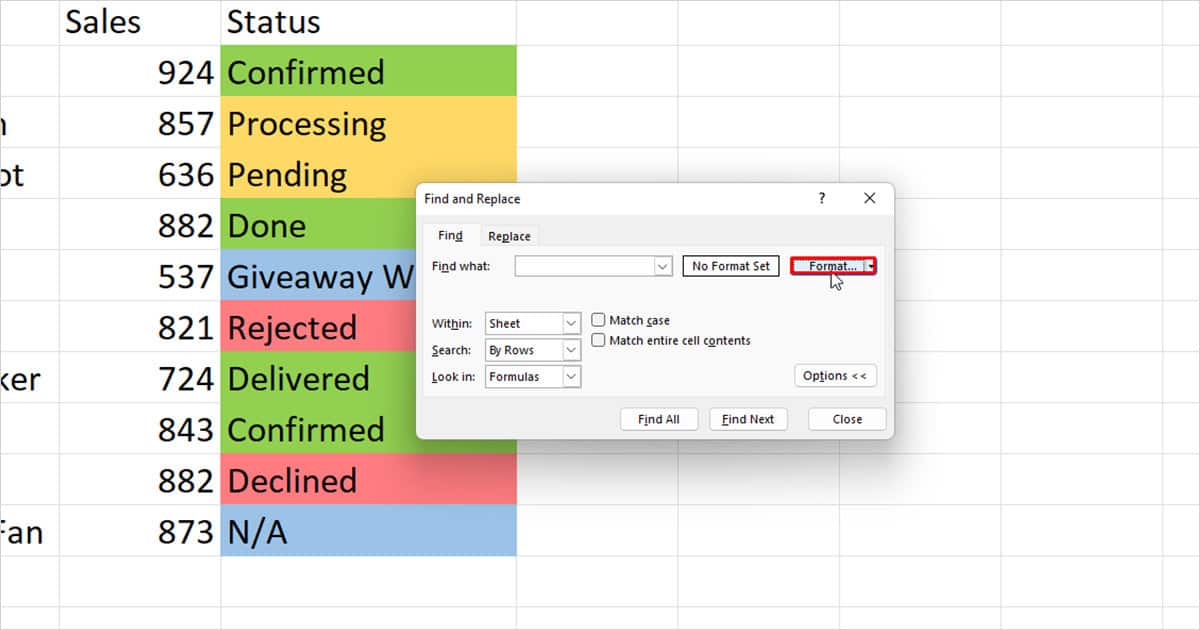
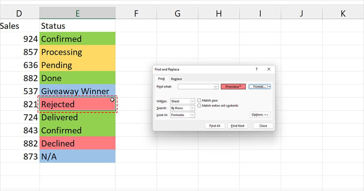
- Next to Find what, select Format.
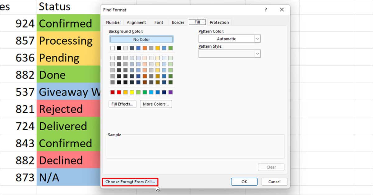
- Select the Choose Format from Cell button.
- From your grid, select a cell with the format.
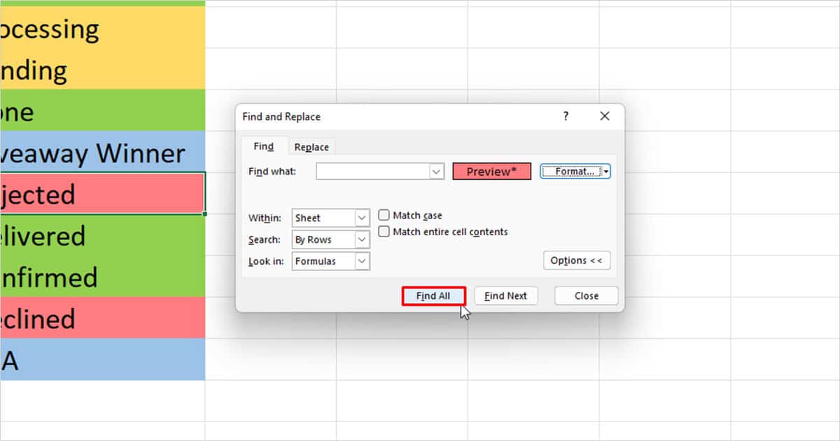
- Click Find All.
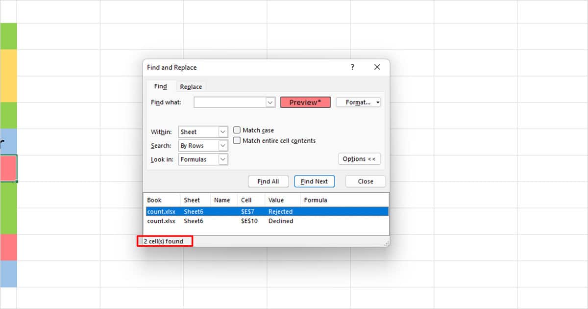
- Check the cell count in the find result.
Filter Values and Use SUBTOTAL Function to Count
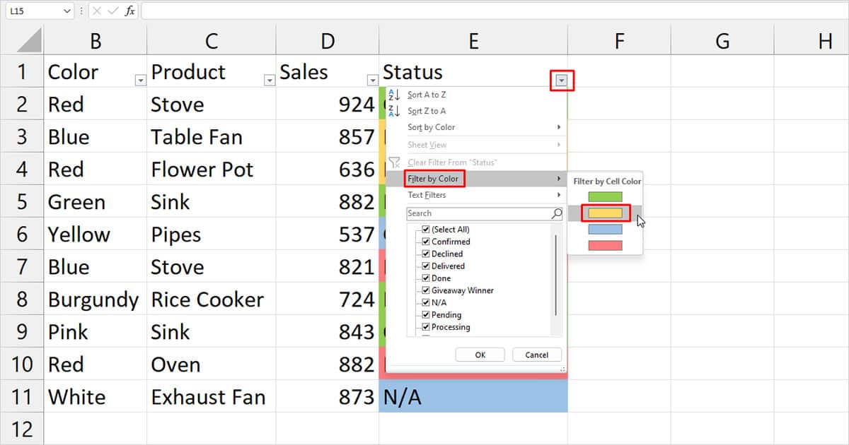
The filter tool in Excel allows you to filter values according to the formatting applied to them. You can filter your data according to the fill and then use the SUBTOTAL function to only count the cells that are on display. For this example, let’s count cells highlighted yellow.
Filter Data
If you have your data in a table, you can skip steps 1, 2, and 3.
- Select your cell range from the grid.
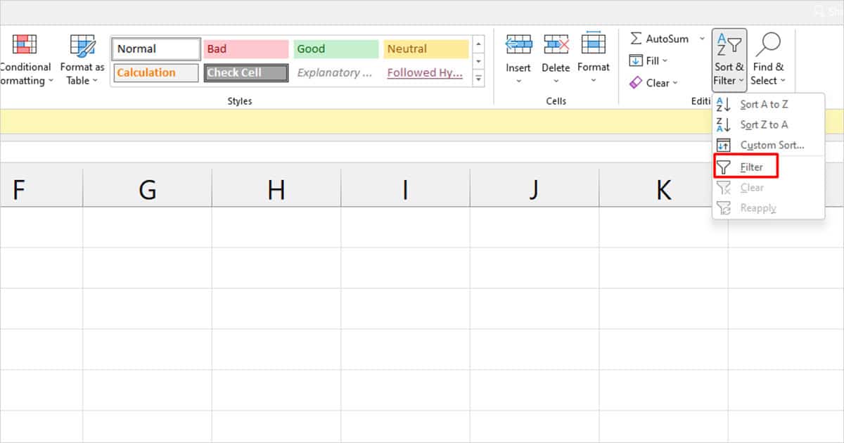
- From the Home tab, select Sort & Filter.
- Choose Filter.
- Select the drop-down icon on the column header.
- Choose Filter by color and select a color if you have multiple.
Use SUBTOTAL to Count
On an empty cell, enter the SUBTOTAL function in the following format:
=SUBTOTAL(103, cell reference)
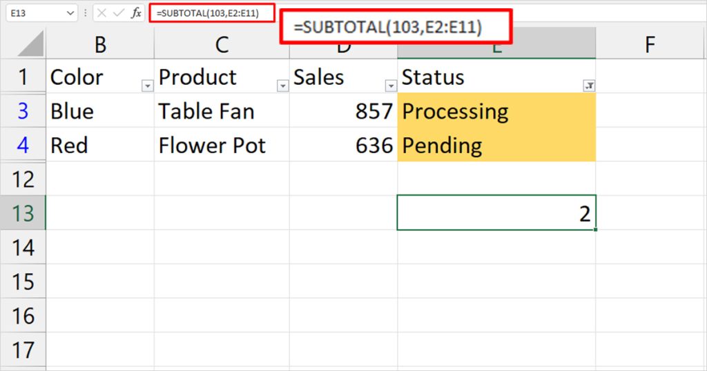
In this sheet, we’re counting the cells that are highlighted as yellow in column E. After filtering our data out, we entered the =SUBTOTAL(103, E2:E11) to count the number of cells.
We used 103 as our function number as it commands the SUBTOTAL function to only count the cells that are not hidden. As we’ve filtered other data out from the display, it will count the cells that are highlighted as yellow.
Use the GET.CELL Macro
You can run the GET.CELL macro by referring to it as a named range. When you run the name in the sheet, rows without a background color will be listed as zero. You can then use the COUNTIF function to count the number of cells that match the result returned by the name.
To explain the application of this method, let’s count the cells highlighted in green.
Define a Name with the GET.CELL Reference
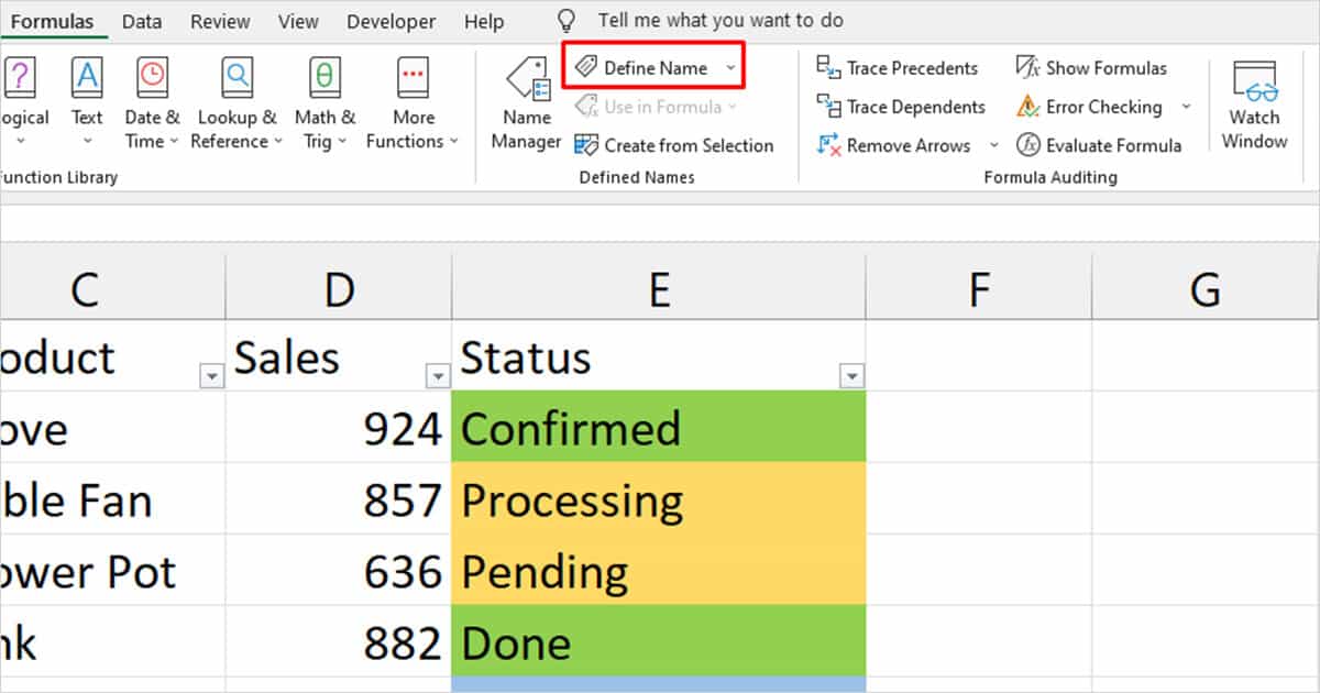
- Open your spreadsheet and head to the Formulas tab.
- In the Defined name section, select Define Name.
- Specify a name. We named our range CountHighlightedCells.
- In the refers to section, enter:
=GET.CELL(38,(range))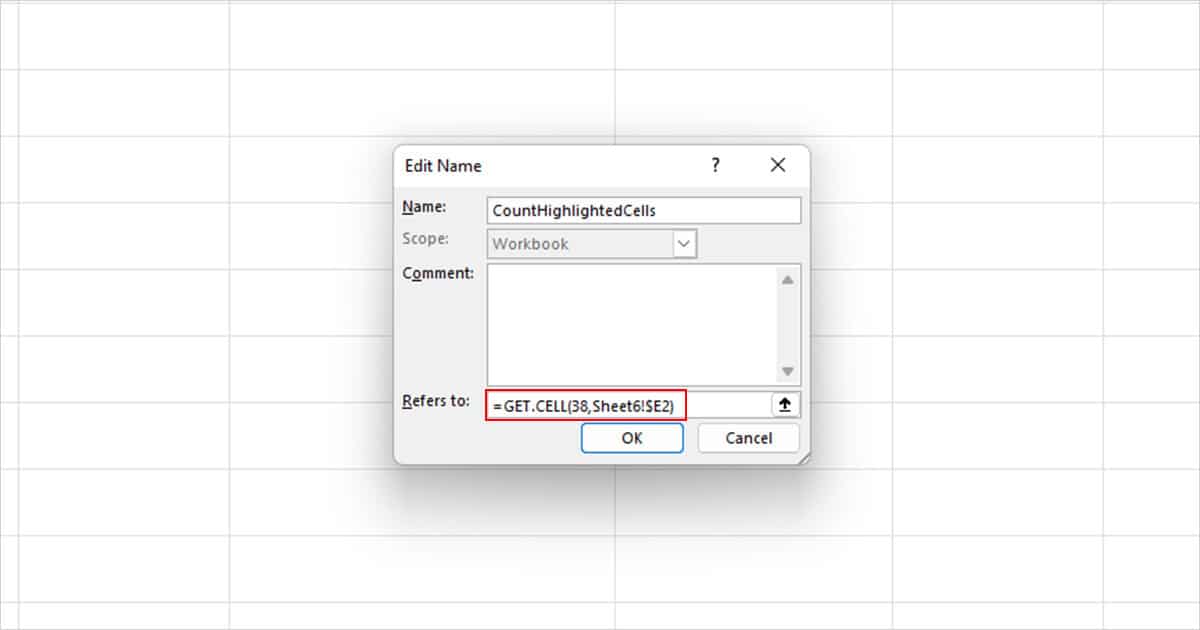
- Click OK.
- Create a new column and enter
=(your named range).
Count Cells Using the COUNTIF Function
After you run the named range, the GET.CELL macro will return a number. You can use this number to count the cells. In a new cell, enter the COUNTIF function in the following format:
=COUNTIF(range, number)
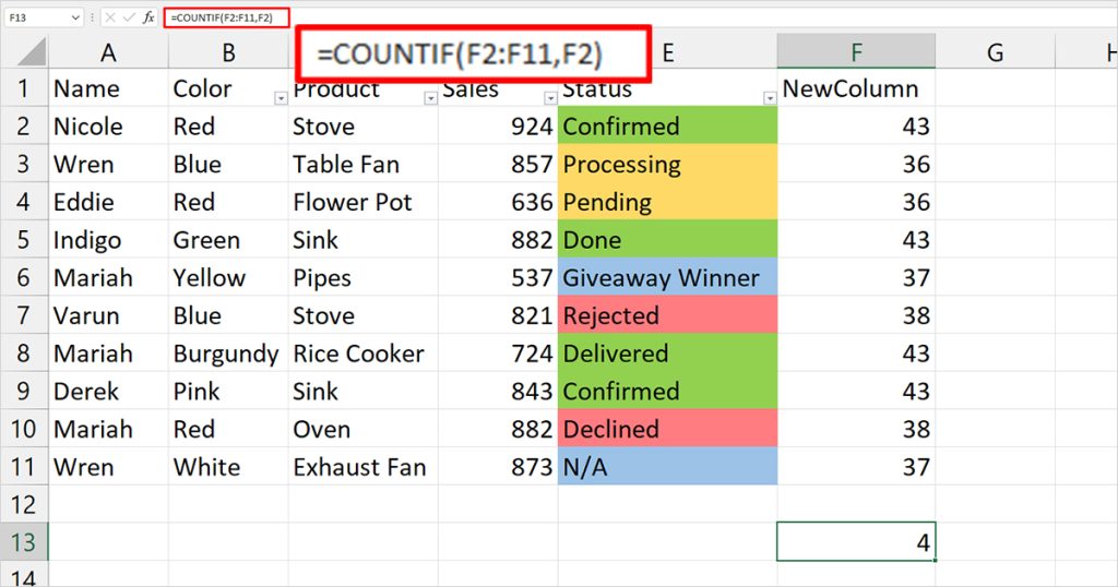
For this example, we’ve counted the cells, color-coded as green. When we ran our range, we got the number 43. Therefore, to command the COUNTIF function to count cells highlighted as green, we entered the following formula:
=COUNTIF(F2:F12,43)
Create a Custom Function Using VBA
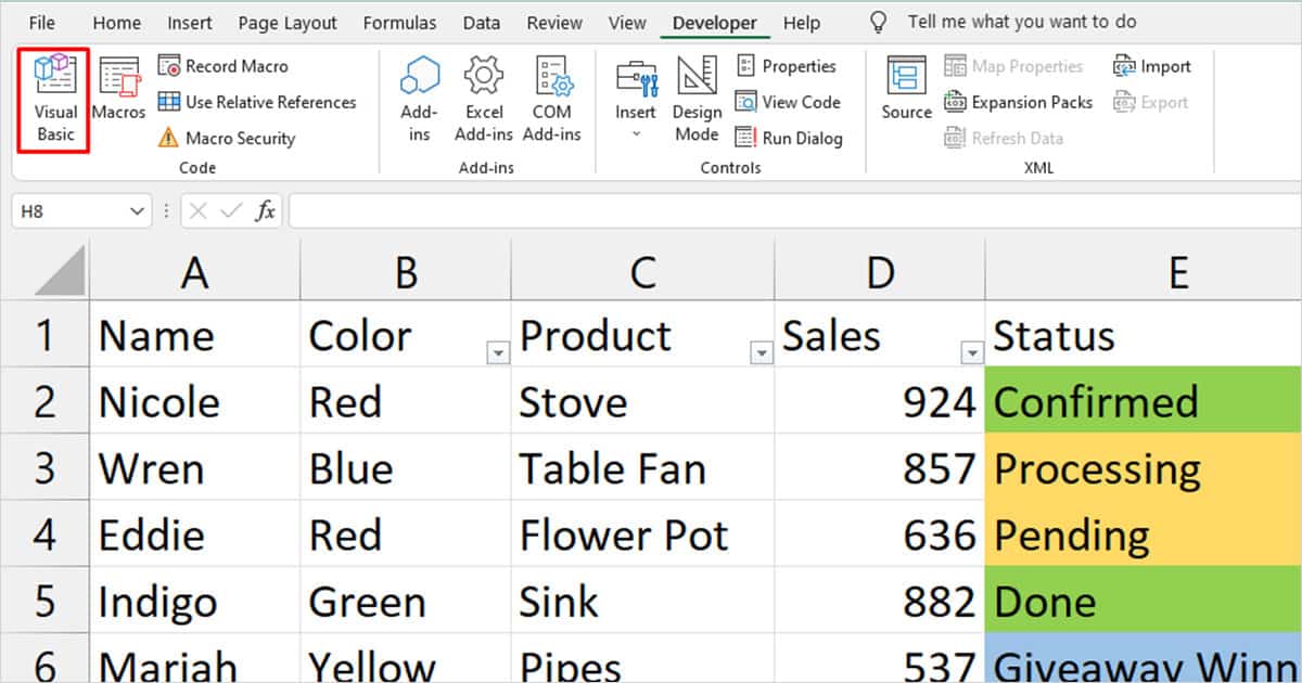
As you may have noticed, Excel really doesn’t have a function to count highlighted cells. This situation calls for a custom Excel function. You can access Visual Basic Editor from the Developer tab. If you haven’t enabled it yet, head to File > Options > Customize Ribbon and enable Developer.
- Head to Developer.
- Select Visual Basic.
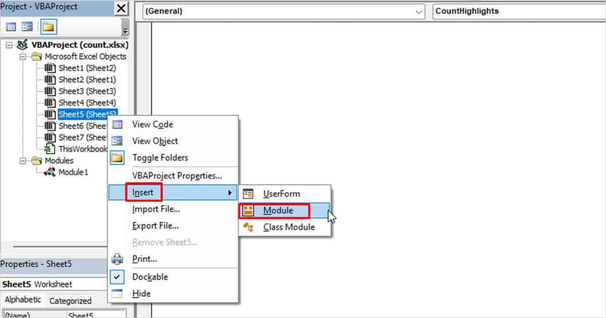
- From the sidebar, right-click on the location you want to insert the function.
- Choose Insert > Module.
- On the window, enter the following code:
Function CountHighlights(CellRange As Range, ref_cell As Range)
Dim Highlight_no As Integer
Dim Result As Integer
Highlight_no = ref_cell.Interior.ColorIndex
Set a = CellRange
For Each a In CellRange
  If a.Interior.ColorIndex = Highlight_no Then
            Result = Result + 1
  End If
Next a
CountHighlights = Result
End Function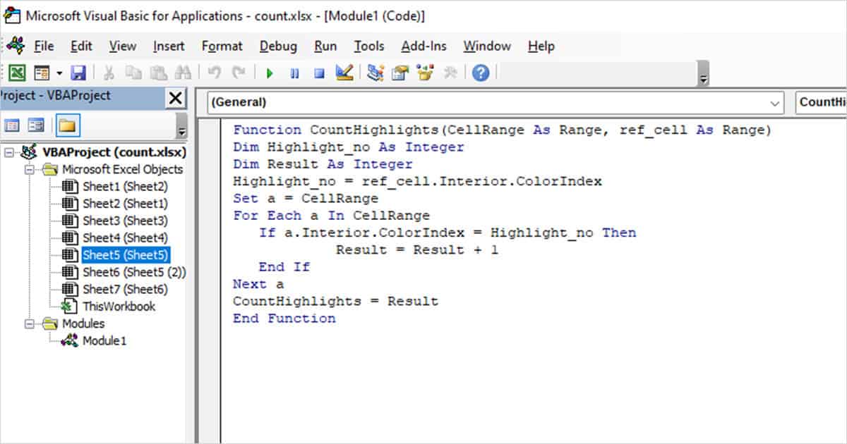
Let’s use our new function to count cells highlighted yellow. First, we highlighted the cell with the exact yellow we’ll be counting. This will serve as a reference for your function. We then entered the following formula:
=CountHighlights(E2:E11,E13)
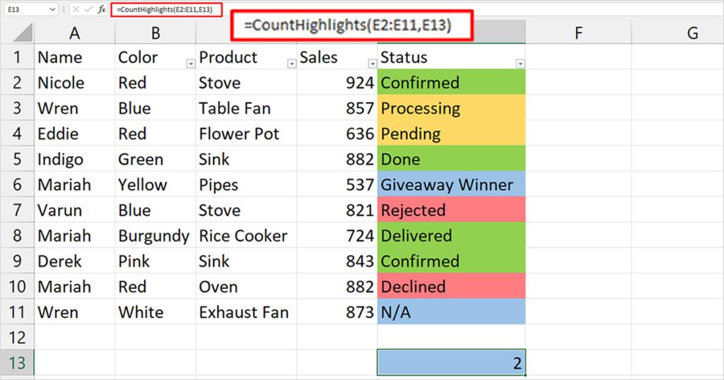
E2:E11 is the range with the highlighted cell and E13 is our reference cell with the same formatting.
How to Count Highlighted Cells with Conditional Formatting?
If you’ve highlighted your cell using Conditional Formatting, except for the second method, the methods we’ve mentioned above won’t work for you. If you specifically want to only count cells that are highlighted using Conditional Formatting, you can run the same formula you used to apply the format under the COUNTIF function.
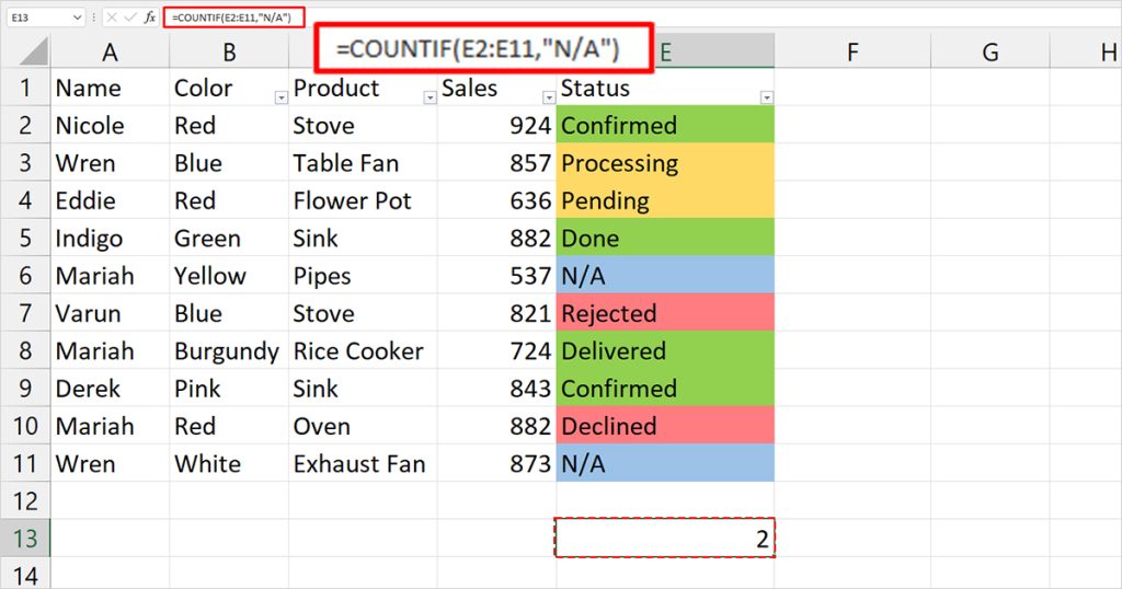
For example, I’ve used the highlighted cells containing N/A in column E with the color blue. To count these cells, I’ll be using the COUNTIF function in the following formula
=COUNTIF(E2:E11, “N/A”)