How to Apply Conditional Formatting Based on a Date

Conditional formatting based on dates makes it easy to highlight and identify specific dates by changing the appearance of a cell according to the specified condition. 

For instance, if you want to highlight payments received in the last week from a datasheet, you can use conditional formatting to identify them easily.

In this article, I’ll walk you through various scenarios where you can apply conditional formatting based on a date.

Conditionally Format Dates Within a Time Period

Excel provides users a built-in option at its Home ribbon to filter and format date cells based on specific filters. You can use these filters to highlight cells within a time period. 

For instance, if you want to filter out products purchased from last week, you can use this option to format your cells and easily highlight the products purchased in the last week.

1. Open the Excel Worksheet and select the cells with dates.  
   
2. Go to Conditional Formatting > Highlight Cells Rules > A Date Occurring.
   
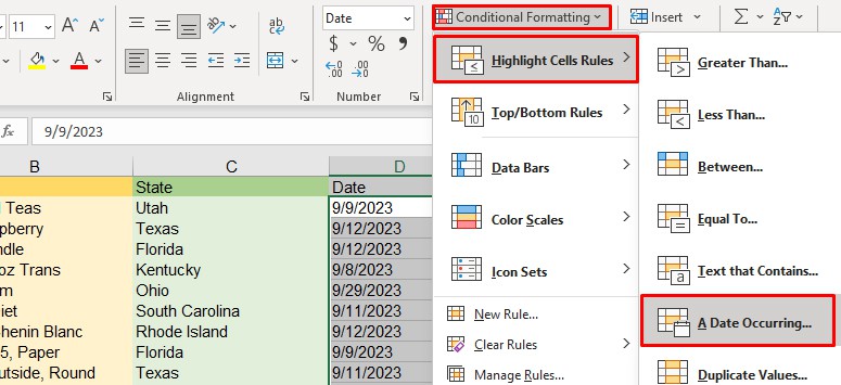
3. Select your preferred date filter from the options box and click OK.
   

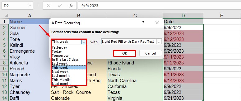
You can repeat the same process to add more formatting filters in the same set of cells. 

Highlight Overdue Dates Using Conditional Formatting

While working with Excel sheets containing payment dates, you can use conditional formatting to determine whether or not a payment is overdue.

For this example, let us consider the due date as after 7 days.

1. Open your Excel sheet and select an empty cell. 
2. Type =TODAY()<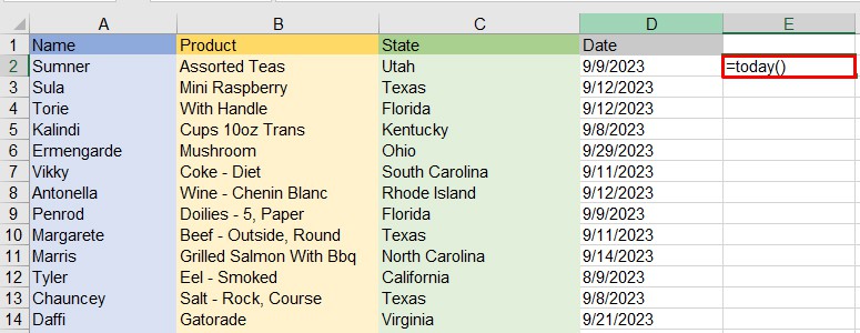
   
3. Click on the cell with the date on it.
   
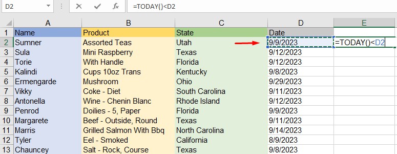
4. Copy the formula. 
5. Select the cells containing the dates. 
   
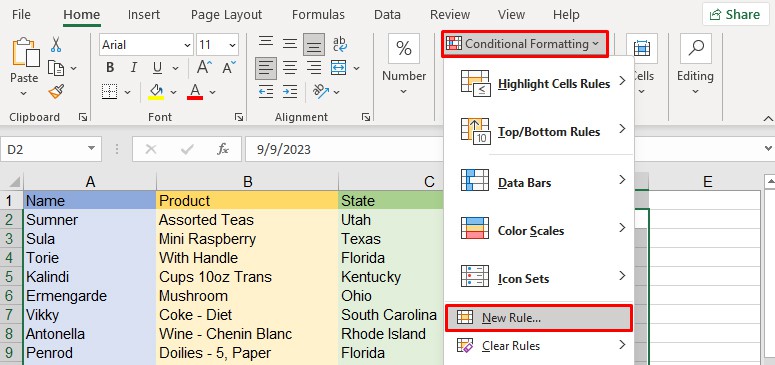
6. Go to Conditional Formatting > New Rule. 
   
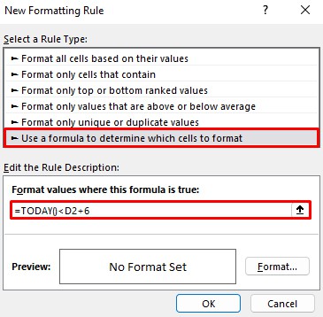
7. Click on “Use a Formula to determine which cell to format” at the bottom.
8. Paste your formula copied from step 4 and add +6 since we’re highlighting dates overdue in 7 days.
   
9. Click on Format, select your preferred color, and click OK.
10. Lastly, click on Apply and click OK. 
    

Conditional Formatting Based on the Expiry Date

You can use the built-in feature from Excel to highlight whether something is expired or getting close to being expired.

1. Open the Excel Sheet and select the cells you want to format. 
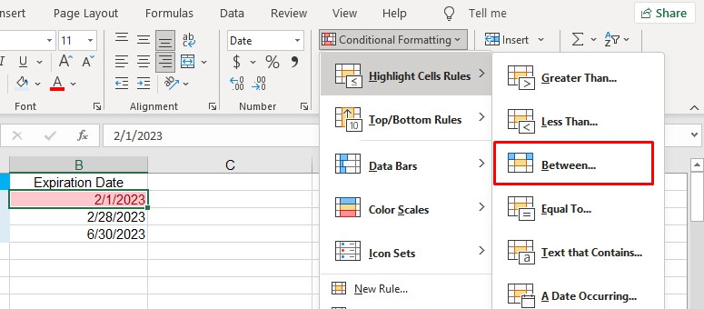
2. Go to Conditional Formatting > Highlight Cell Rules.
   
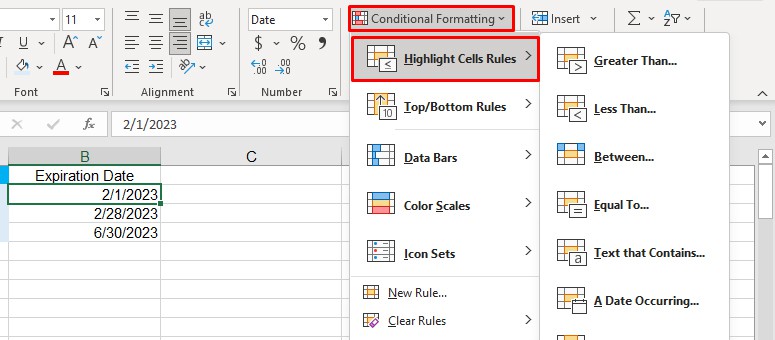
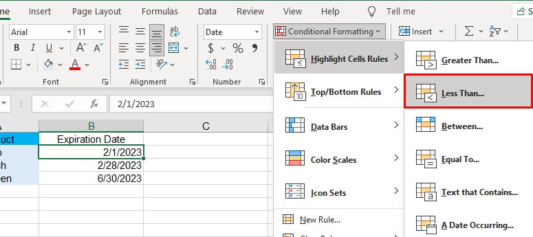
3. Now, click on Less Than.
   
4. Type in =today() and select the highlight color. This will highlight the cells that fall today.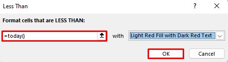 
   
5. In the same range, layer in a second condition by repeating Step 2. 
6.  Now, Click on Between. 
   
7. In the parameters add =today() and =today()+30 and select the highlight color. This will highlight the cells that fall between today and 30 days.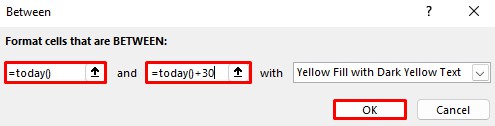 
   
8. In the same range, layer in a third condition by repeating Step 2.
9. Now, Click on Greater Than.
   
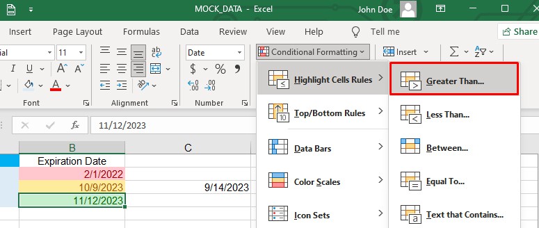
10. Type =today()+30 and select the highlight color.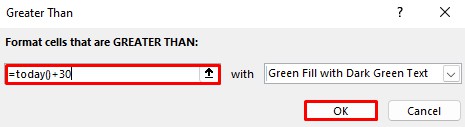 
     

Conditional Formatting Based on the Date in Another Cell

You can also use conditional formatting if you want to highlight dates based on whether they fall within a specific date range.

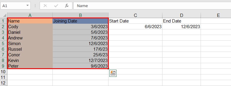
Say you need to identify which employees have joined your company within a specific date range. With the help of conditional formatting you can compare date ranges to highlight cell data.

1. Open the Excel Sheet and select the cells where you want to apply conditional formatting.
   
2. Go to Conditional Formatting > New Rule and select Use formula to determine which cells to format as shown in earlier methods.
3. Enter the formula with reference to your cell numbers.
   =AND($B2>=$C$2,$B2<=$D$2)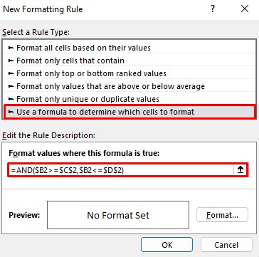
   
4. Click on Format, go to Fill, select your desired highlight color, and click OK.
5. Click OK again on the new screen and finally click on Apply and OK. 
   

Now, the dates that fall under your specified range will be highlighted.

Highlight Days in Excel

If you’re looking to highlight any day on Excel from a given set of data, you can add conditional formatting to it using a formula. 

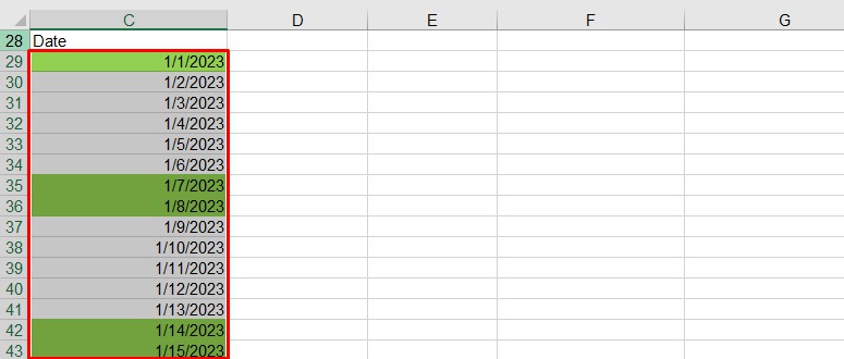
In the example below, I’ll be highlighting only weekends.

1. Open the Excel Worksheet and select the columns.
   
2. Go to Conditional Formatting > New Rule.
   
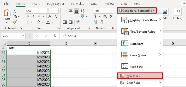
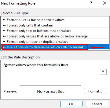
3. Click on “Use a Formula to determine which cell to format” at the bottom.
   
4. Add this formula with reference to your data cells.
   =WEEKDAY(C29,2)>5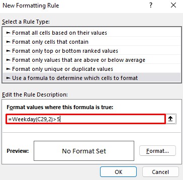
   
5. Click on Format, and open the Fill tab.
6. Select your highlight color and click OK.
7. Lastly, click Apply and OK to save your changes. 
   

Remove Conditional Formatting

We’ve covered applying conditional formatting in the section above. Now, what if you want to remove conditional formatting? Let’s take a look at how you can do it. 

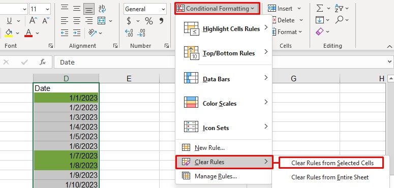
1. Open the Excel Sheet. 
2. Select the cells where you want to remove conditional formatting.
   
3. Go to Conditional Formatting > Clear Rules > Clear Rules from Selected Cells.