How to Add Error Bars in Excel

Statistically, error bars represent the precision of your data. If your chart has metrics like standard deviation, confidence intervals, and standard error, inserting an error bar will give you a general idea of the spread of your data.

You can insert Error bars on Excel’s charts including 2D columns, bars, 3D bars, and even scattered plots.

KEY TAKEAWAYS

• You can insert error bars for a set fixed width, standard deviation, percentage, and standard error.
• You can customize error bars by entering positive and negative error amounts.
• You can format your error bar’s line direction and end style.

How to Add Error Bars in Excel

You can insert error bars using two methods in Excel. You can either add the element from the Design ribbon, or directly from the chart. Once you enter the error bar, you might have to format the error bar’s direction, end, and the error amount according to your needs.

From the Ribbon

This chart represents the standard deviations of five random data sets in three trials. Here’s how you can insert error bars from the Design ribbon.

1. Go to the Design tab.
2. In the Chart Layout section, click Add Chart Element.
   
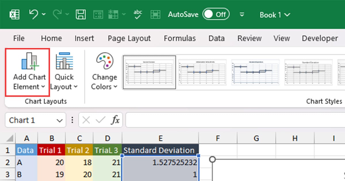
3. Select Error Bars.
4. As our data represents standard deviation, we chose Standard Deviation.

From the Chart

Once you click on the chart, you can add different elements such as Axis Titles, Data Labels, and Error Bars.

1. Click on the chart.
2. Select the plus (+) icon on the right.
   
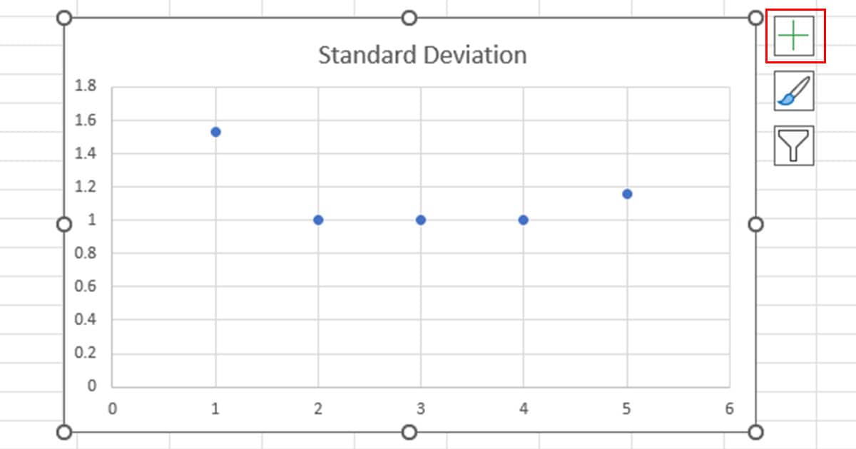
3. Under Chart Element, select the box next to Error Bars.
   
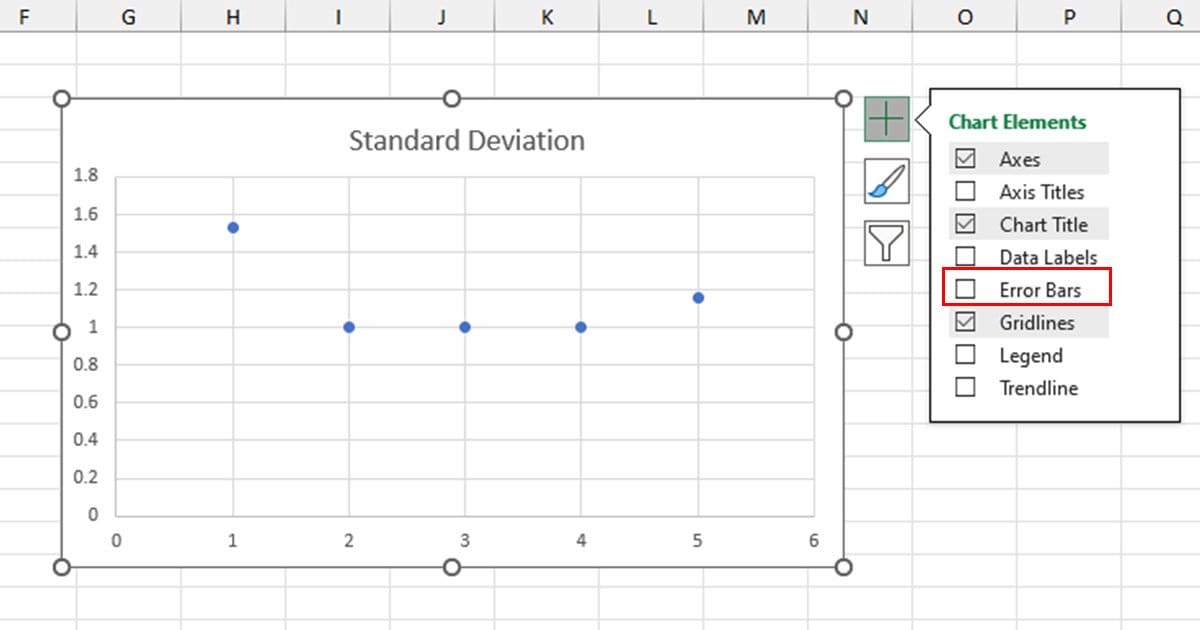
4. Choose an option.

Customize Error Amount for Error Bars

Excel gives you the option to create error bars through set error amounts for Standard error, Standard Deviation, and Percentage and even insert a Fixed Value. 

However, you can also set a positive and negative error value to customize your error amount.

1. Select your chart and click on plus (+).
2. Choose Error Bars > More Options.
   
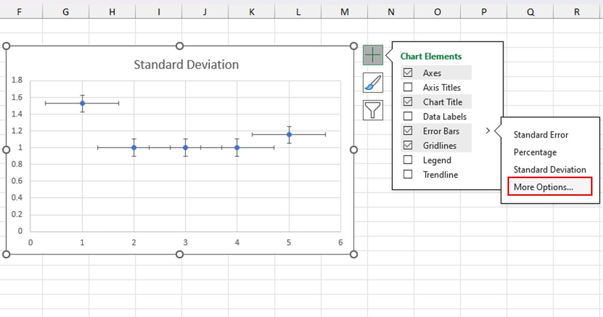
3. Under Error Amount, enter either a Fixed value, Percentage, or Standard deviation.
4. If you want to further customize the amount, select Custom and click on Specify Value.
5. In the Positive Error Value section, reference your error amount.
   
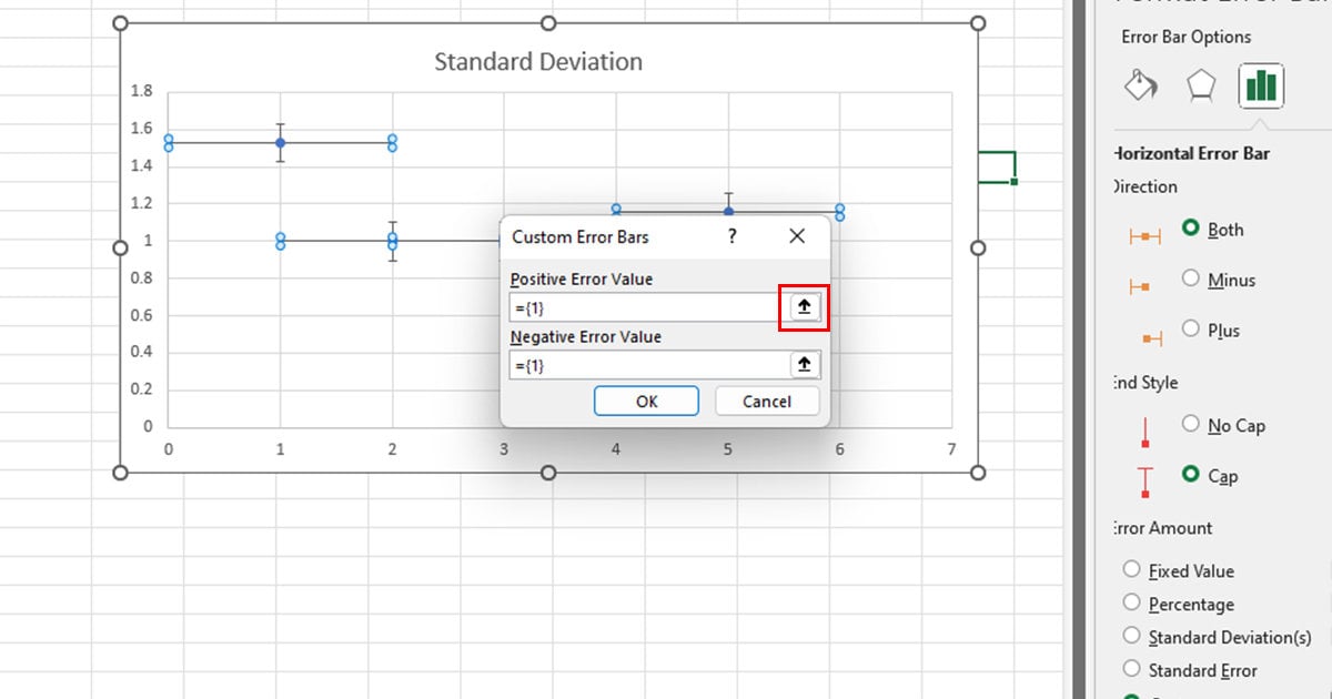
6. Click OK.

Format Error Bars

By default, Excel formats the error bars to be in both directions with a cap end style. However, when you’re inserting error bars for illustrations such as a box plot chart, you will need to change the direction and the end style of your error bars.

You can format your error bars in Excel to fit into these adjustments.

1. Select your chart and click on plus (+).
2. Go to Error Bars > More Options.
   
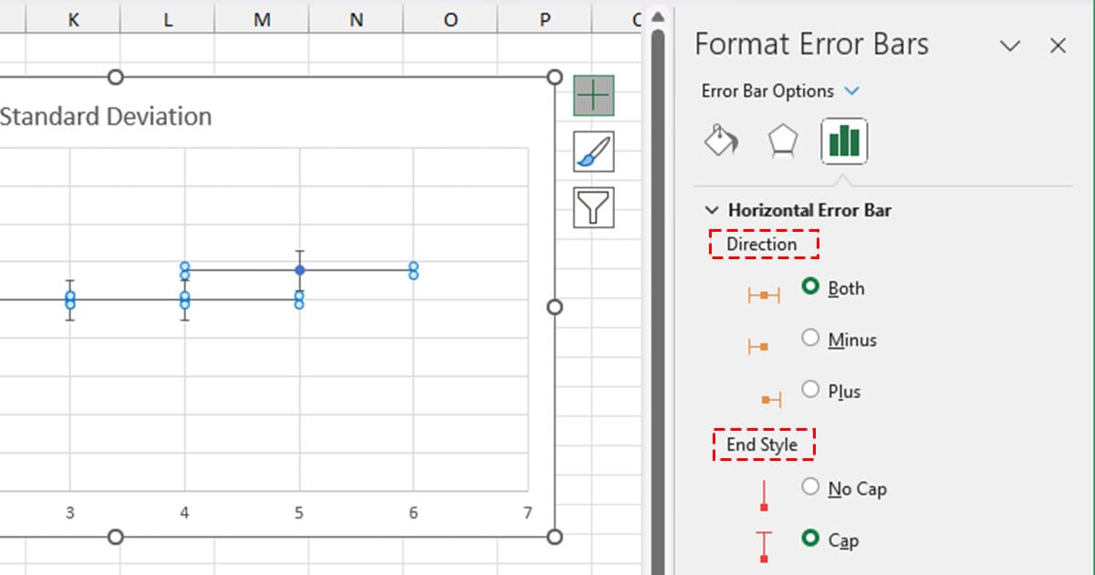
3. Under Vertical Error Bar, first choose the direction of your bar.
4. Next, choose if you wish the end to have a Cap or No Cap.
   

Change Fill and Line Style for Error Bars

As aesthetics play a huge role when presenting data, you may want to beautify your error bar. In Excel, you have the option to change the error bar line by setting different colors, adjusting transparency, arrow size, and so on.

1. Right-click on your error bar.
2. Choose Format Error Bars.
3. From the Error Bar Options, select the Fill Bucket icon.
   
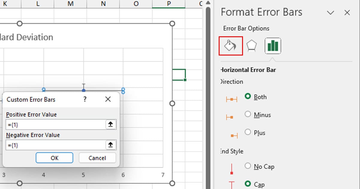
4. Choose a Line style.
5. Select the color, transparency, and width. Choose from the additional stylistic options to beautify your error bar.

How to Delete Error Bars in Excel

To remove error bars in Excel, you can simply disable them from the add chart elements view.

1. Select your chart and click on the plus (+) sign.
2. Uncheck the box next to Error Bars to disable it.