The COUNTIF and COUTIFS functions are one of the count functions, under the statistical category in Excel. You will get to the set criteria and, the function will only count the cells that match your set criteria. The use of wildcards is one of the most handy features in my opinion. This gives you a wider scope to count your desired values.
Although you can get the most use out of the COUNTIF function as it is, The COUNTIF function is limited to one criterion. To set multiple count criteria, you can always nest multiple COUNTIF functions inside each other. However, this makes your formula look quite long. To avoid this, use the COUNTIFS function instead for when you wish to count cells that pass multiple criteria.
You may now be wondering how the COUNTIF and COUNTIFS functions differ. Well, as COUNTIFS accepts multiple criteria, its syntax ends up looking a bit different than COUNTIF. This makes the application of these functions unique from each other.
Arguments Used in COUNTIF and COUNTIFS
To put the arguments in both, COUNTIF and COUNTIFS functions in simple terms, they’re basically asking you where to find your value, and what to find.
Remember, If you’re passing a text value as the criteria put them in double quotes. Both functions also take named ranges when setting reference values. Here are how the functions are written in the following format when constructing a formula:
COUNTIF
=COUNTIF(range, criteria)COUNTIFS
=COUNTIFS(criteria_range1, criteria1,[criteria_range2], [criteria2]...)Use of Wildcards
The count functions accept the use of wildcards, including the asterisk (*), question(?), and tilde symbols(~). These wildcard characters are dismissed as actual values in Excel and are seen as commands. Each of these characters has a unique function, and can either be used on their own or paired with the set criteria.
Asterisk (*)
Asterisk is used to select all values that start or end with the entered letter. For this, the placement of the wildcard is important. For example, If your criterion is “*a”, the function will count values that have the last letter as “a” or “A”, like “Canada” and “Sandra”. Similarly, if your criterion is “a*”, the function will count values that start with “a” or “A”, like “Asmi” and “Arizona”.
If you use an asterisk on its own, it will count all values in the range.
Question (?)
The question symbol acts as placeholder text when entering a criterion inside the function. If you’re confused with the spelling of the criterion or want to count all same-length values that begin with the same letter, you can swap out the letters in the middle with the question mark wildcard. For example, if your criterion is “T?m”, it will count both cells like “Tom” and “Tim”.
Tilde (~)
Tilde is used when you don’t want to use the wildcard symbols as a wildcard. You may sometimes need to count cells that contain asterisks or questions in them. As these characters are wildcards, you will have to enter a tilde before you enter them to override their function as a wildcard.
Examples of the COUNTIF and COUNTIFS Function
The application of these functions is pretty similar. To put it into comparison, If COUNTIF counts the number of students who have passed a subject, then COUNTIFS counts the number of students who passed all subjects. Except for the number of criteria allowed, these functions are exactly the same.
Let’s put both of these functions into application to count several occurrences.
Example 1: Count How Many Times a Value is Repeated
Take a look at this data table.
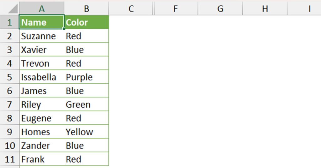
Notice how some values have been repeated a number of times. We can use the COUNTIF function to count the repetition of a value. We will be using the COUNTIF function to see how many times the value, “Red” is repeated in the range B2:B11.
In cell E5, we entered the following formula:
=COUNTIF(B2:B11, “Red”)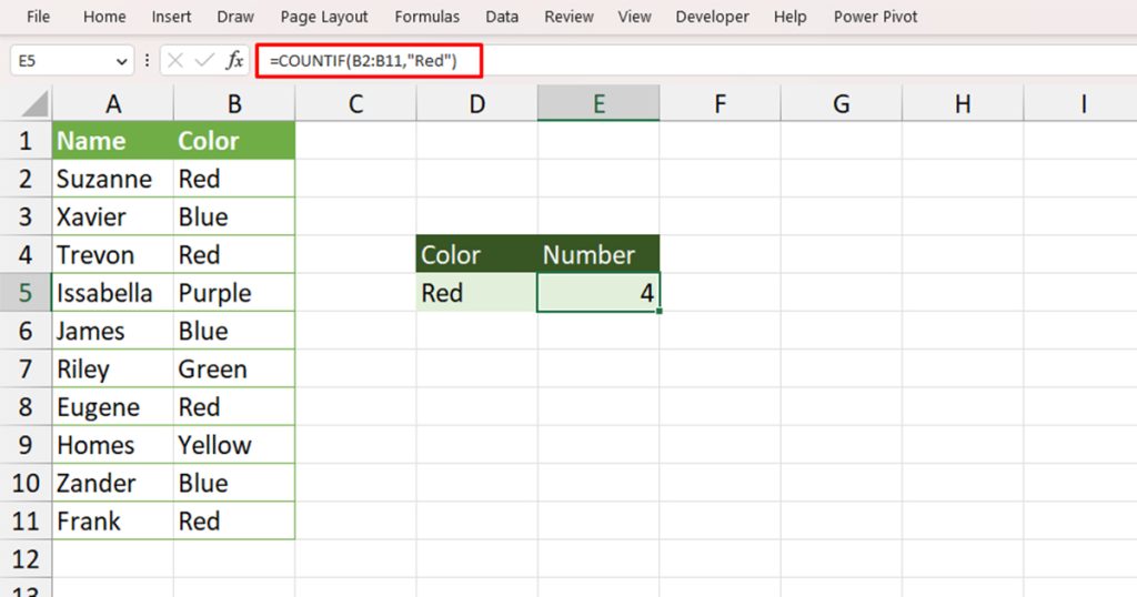
Example 2: Count All Texts That Begin with “A”
In this table, we have the names of people in column A.
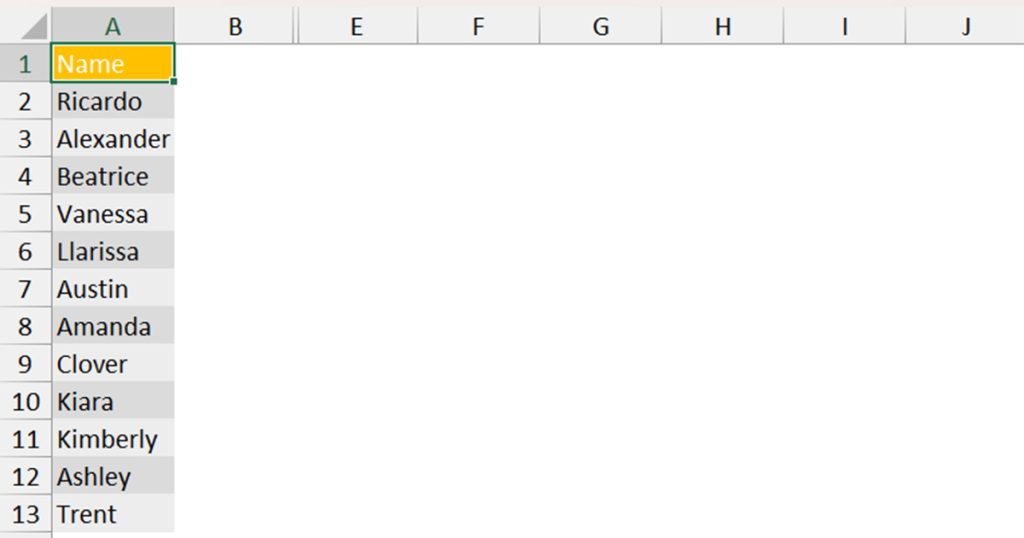
We can use the COUNTIF function to count the names of all individuals whose names begin with the letter “A”.
We will be using the asterisk (*) function while setting the criteria inside the COUNTIF function. In cell D6, we entered this formula:
=COUNTIF(A2:A13,"A*")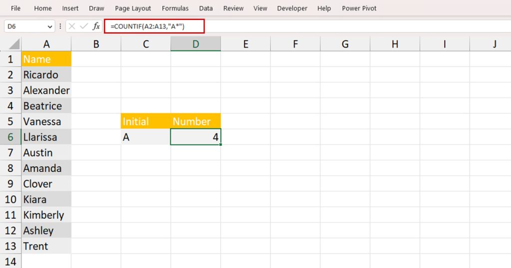
Example 3: Count Numeric Inequalities
This table represents the grade sheet of a class.
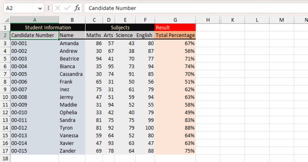
We have to make three counts, count the total number of students that passed and students who scored less than 60% on average. We will be using both COUNTIF and COUNTIFS to calculate each of these occurrences. Additionally, we will be using the greater than (>), less than (<), and equals operators to set our condition.
Count Students Who Passed
The total passing percentile of this exam is 40%. However, there’s a catch. Even if the total score averages out to be more than 40%, they will still be marked failed if they scored less than 40 in one subject. To accommodate each criteria, we will be using the COUNTIFS function.
This will count cells that have scored at least 40 on all tests and have a percentile of at least 40.
=COUNTIFS(C3:C17,">=40",D3:D17,">=40",E3:E17,">=40",F3:F17,">=40",G3:G17,">=0.40")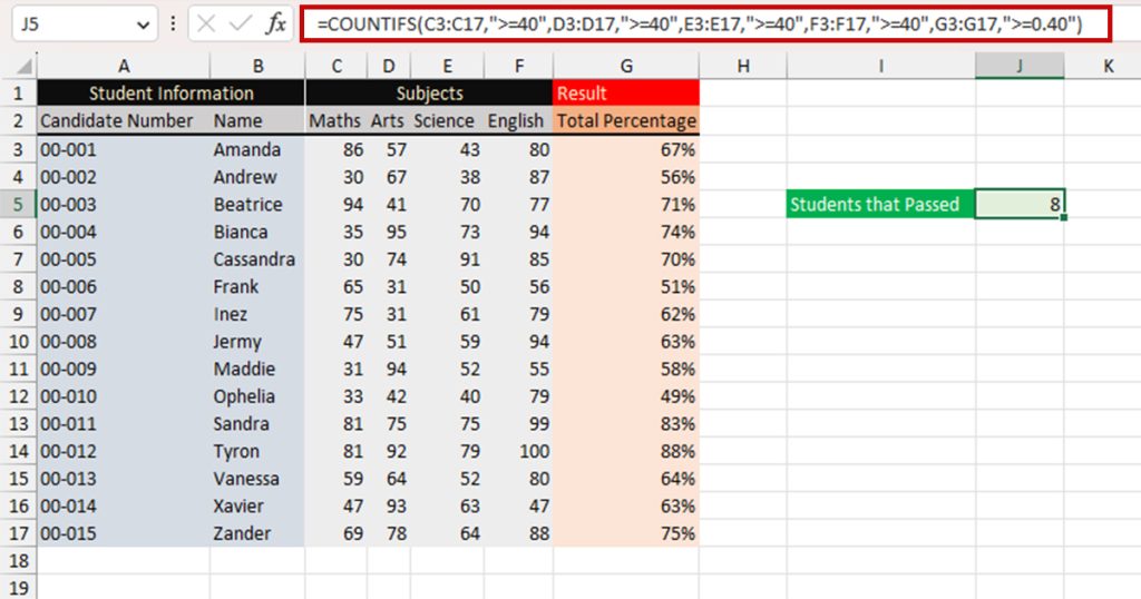
You can count the number of students who failed by subtracting the total number of students from the students who passed. If you try to calculate this value by using the less than (<) operator, you will get 0 as a result. This is because each range has at least one number that is more than 40. All criteria must be true inorder for COUNTIFS to make a count.
Count Students Who Scored Less than 60%
Let’s assume you, as the school administrator wants to organize a special class for students that scored less than 60% on average. We will be using the COUNTIF function to count this occurrence.
=COUNTIF(G3:G17,"<60%")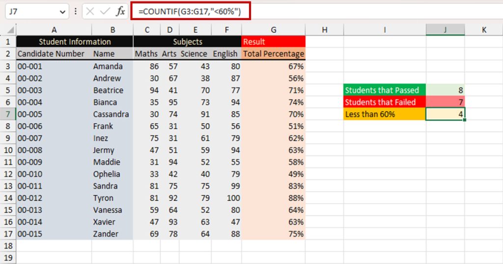
Example 4: Count Cells that are Empty/ Non-Empty
Although you have COUNTBLANK and COUNTA functions to count cells that are empty and non-empty respectively, you can also use COUNTIF to count both of these occurrences.
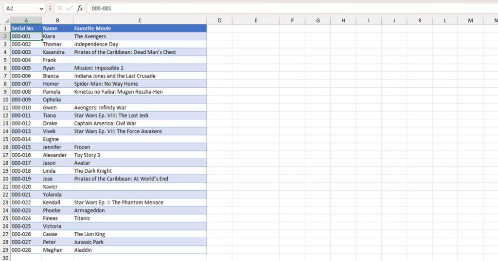
This table holds the favorite movies of 28 individuals with their serial numbers. Unfortunately, as you can see not everybody has given out the names of their favorite movie. Let’s use the COUNTIF function to check how many people submitted the name of their favorite movie, and how many remain.
Count Non-Empty Cells
We will be using the not equals to (<>) operator in this formula. In our formula, we will pass the criteria as counting cells that are not equal to “”, which indicates a blank cell.
=COUNTIF(C2:C29,"<>"&"")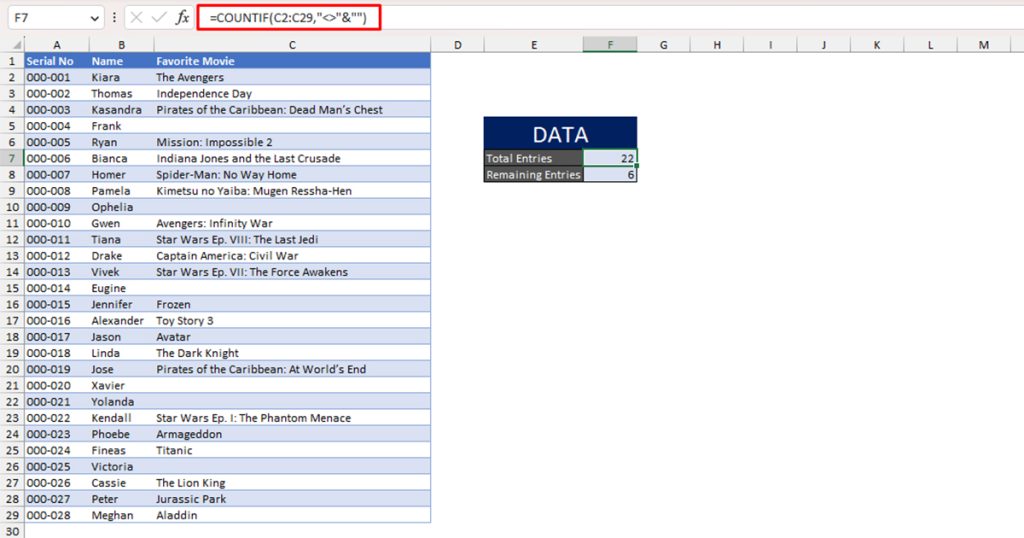
Count Empty Cells
Constructing this formula is rather simple. All you have to do is set “” as your criteria in the COUNTIF function.
=COUNTIF(C2:C29, "")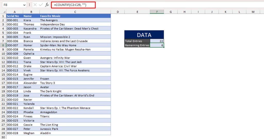
Example 5: Count Cells with Similar Values
For our next example, we will be using the question mark wildcard, (?) to count cells with similar values from the following table:
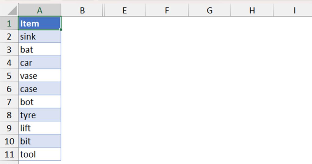
Column A holds 10 values (excluding the header). Let’s use the question wildcard to count values that are similar to bat and bot. If you notice, the only character difference is the one in the middle.
In this case, we will be using the ‘?’ symbol in place of the middle character to assign the COUNTIF function to count all three-character cell content that starts with b and ends with t.
In cell D5, we designed the COUNTIF function in this way:
=COUNTIF(A2:A11,"b?t")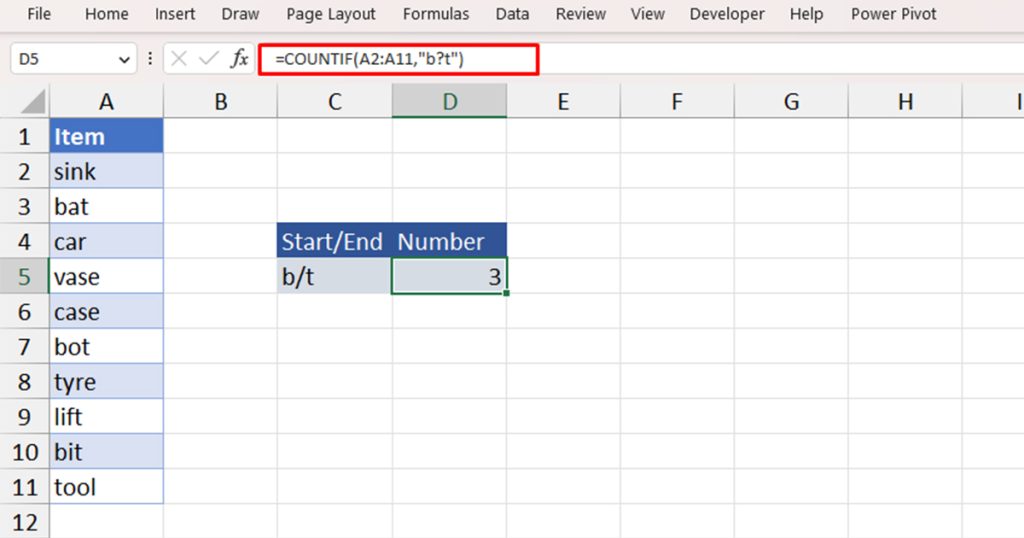
Example 6: Count the Wildcard Characters
What if you actually need to count the wildcard characters? Excel would not treat your characters as values but as wildcards. Fortunately, this is a well-thought-out phenomenon. You can use the tilde character before entering the wildcard. This will assign Excel to treat the character as a value, not a wildcard.
We can construct a formula that counts the total number of times the asterisk symbol (*) has been repeated in a range in this manner:
=COUNTIF(A2:A21,"~*")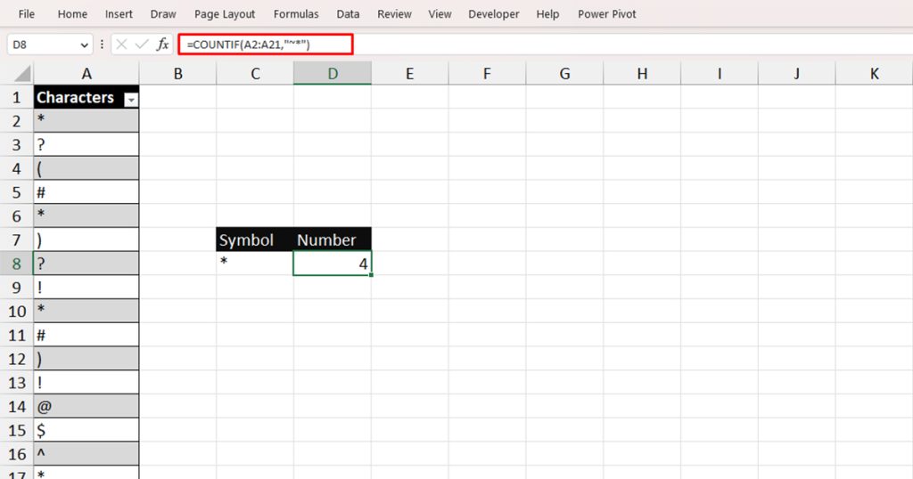
Example 7: Count Cells with Error Value
You can pass the name of your error as your criteria in the COUNTIF function, and the function will count the number of occurrences for you.
Here, we have a range of data. Some cells in the range, however, have #VALUE! error in them. Let’s construct the COUNTIF function to count cells with the #VALUE! error.
=COUNTIF(C2:C11,"#VALUE!")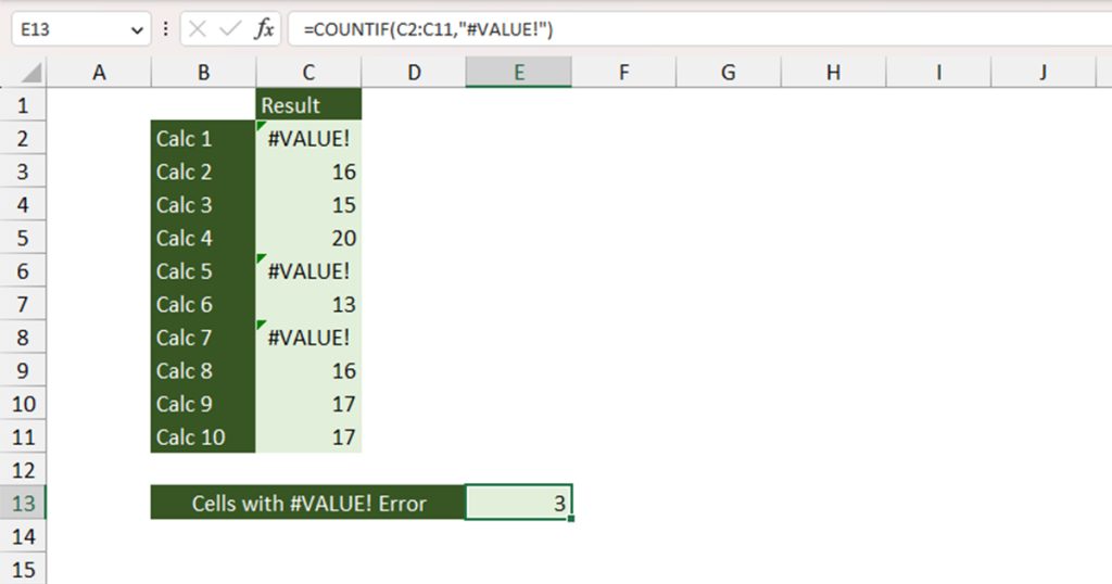
Example 8: Count Values with Specific Criteria
Here is the sales sheet for a certain month of this year.
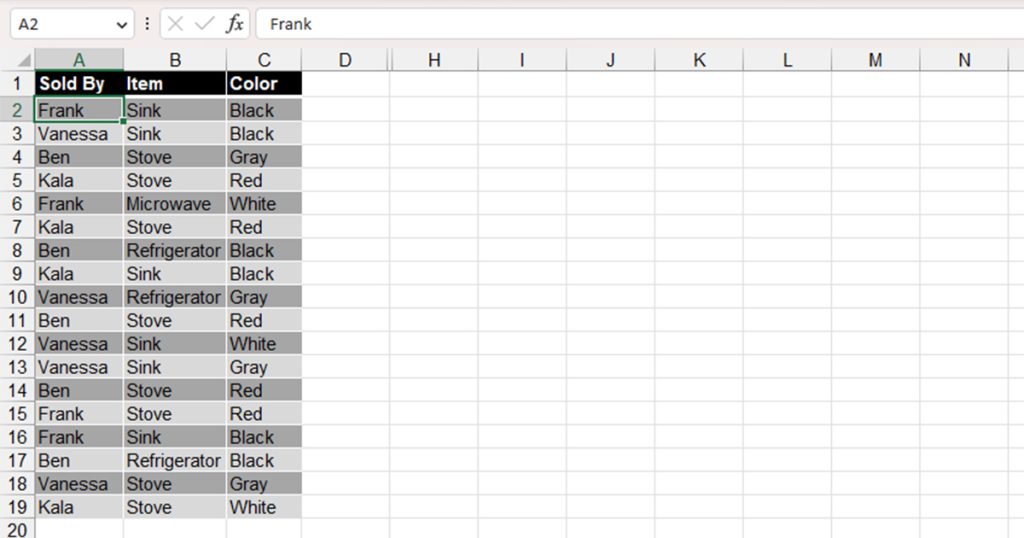
Say your manager asked you to check the demand for the “Red Stove” to see if they should get more in stock. Fortunately, you’re well aware of the COUNTIFS function and use the following formula to count the occurrences of “Red Stove” in the sales sheet:
=COUNTIFS(B2:B19,B4,C2:C19,C5)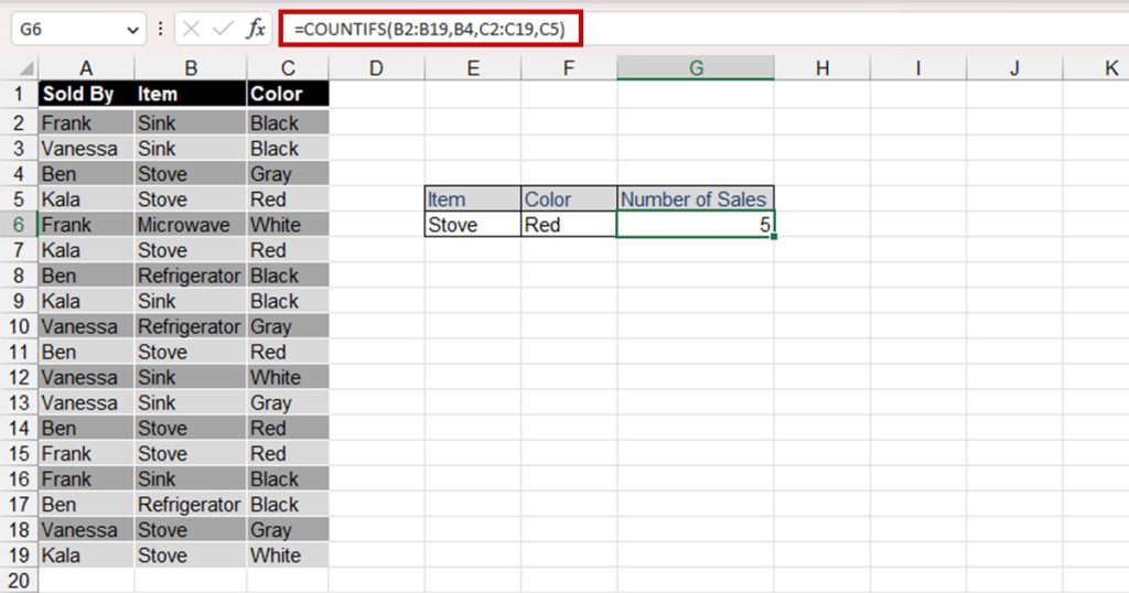
Why am I Getting the “You’ve entered too few arguments for this function” Error?
This error is not specific to these functions. When you fail to enter the required arguments in a function, Excel triggers the “You’ve entered too few arguments for this function” error.
The COUNTIF and COUNTIFS function requires two arguments to return a result. If you fail to insert any one of the first two criteria, the range, and the first criteria, Excel will display the above-mentioned error.
If you’re just starting out in Excel and need help with passing arguments, you can use the Insert Function (Shift + F3) tool to create formulas in your sheet.