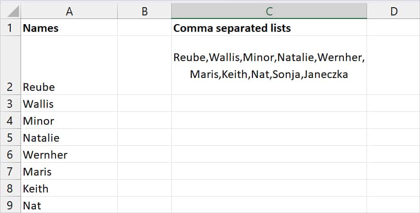
If you have large lists of data in rows, you won’t be able to see the entire data in one view. But, if you format those values into a single row separated by a comma, you could easily expand the view. As you can see in the given example itself, comma Separated Lists take up a lot less space.
To convert your existing lists into comma-separated values, we will use two easy Excel functions and an Ampersand Symbol. You could follow any one method according to your data size.
Using Ampersand (&) Symbol
If you have small data to convert into comma-separated values, you could use the Ampersand (&) Symbol. Excel’s (&) operator joins texts from separate cells. Here, you can insert a (,) comma delimiter while combining texts.
Example: Let’s say you need to format the cell value of A6 and A7 into comma-separated lists. For this, your formula using the Ampersand symbol would be
=A6&“,”&A7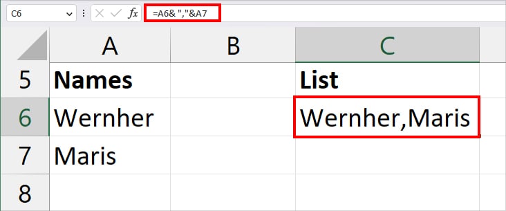
In the formula, each Ampersand symbol combines the text strings of A6 and A7. Similarly, since we have specified “,”, the formula will return a comma in between the texts.
Using TEXTJOIN Function
Excel’s TEXTJOIN function returns the joined texts of different cell ranges along with a delimiter you specify. Usually, I use the TEXTJOIN function to combine texts of separate columns along with a delimiter. However, you can also use this function to return values of multiple rows into one row divided by a comma.
Note that you can access and use the TEXTJOIN function only from Office 2019 onwards or on Office 365.
Syntax: TEXTJOIN(delimiter, ignore_empty, text1, [text2],...)While using the TEXTJOIN function, you must mandatorily pass down three arguments. Let’s see what each argument refers to.
- delimiter: characters like space, comma, /, &, – to insert in between the texts [required]
- ignore_empty: specify whether to disregard the empty cells or not [required]
- TRUE will empty cells
- FALSE won’t ignore blank cells
- text1: words or cell references to join [required]
- text2: extra text strings or cell ranges to join [optional]
Now, let’s take a look at the example of using the TEXJOIN function to convert the list into comma-separated values. Here, we have a list of First Names in Column A. To combine all names and separate them with commas, we entered the formula as
=TEXTJOIN(",", TRUE, A2:A11)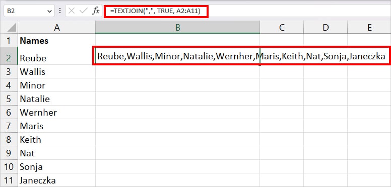
In the above formula, we have passed down a comma as a delimiter “,”. Similarly, the TRUE argument will ignore any blank cells within the cell ranges. As an output, it’ll return all the values from Cell A2 through A11 with a comma in Cell B2.
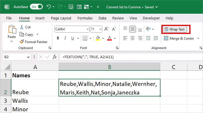
After you get the result, it will most likely span in the next columns. For this, you can use Wrap Text to fit everything within a cell. On Home Tab, navigate to the Alignment section and click on Wrap Text Icon. If needed, adjust the row height too.
Using CONCATENATE Function
Since the TEXTJOIN function is not available in older Excel versions like 2016, you could use the CONCATENATE function as an alternative. Excel’s CONCATENATE function is also built to combine two or more text strings. It basically functions the same as the (&) Ampersand Symbol. Here, you can pass down a particular delimiter while merging the values.
Syntax: CONCATENATE(text1, [text2],...)CONCATENATE function only takes multiple text strings as arguments. Compared to TEXTJOIN, this function can be a bit tiring to join texts with a delimiter. This is because you would have to manually enter each delimiter in the formula. Also, when you pass down delimiters, you must strictly enclose them inside the double quotation mark.
Suppose, you need to combine texts of cells A2, A3, A4, and A5 with a comma in between. For this, your formula would be
=CONCATENATE( A2, ",", A3, ",", A4,",", A5)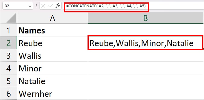
In the formula, A2 refers to text1, “,”, as text 2, A3 as text 3, and so on. As a result, it returns Reube,Wallis,Minor,Natalie.
In case you wish to add spaces in between these comma-separated values, you could enter this formula.
=CONCATENATE( A2,", ", " ", A3, ",", " ", A4,",", " ", A5)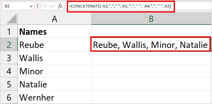
Now, in this formula, we have passed down to “ ” after the comma to return a space. So, your result will be Reube, Wallis, Minor, Natalie.