CHOOSE is a lookup function in Excel, typically used to extract a value from the set list of ranges, passed as arguments. While the function may not be used as much on its own, nesting it with other functions can create help you automate certain calculations.
The CHOOSE function isn’t dynamic in nature meaning, that if you add to the specified list in your spreadsheet, the function will not automatically update the formula. Therefore, if you add to your list of data, be sure to manually update it in the CHOOSE function.
Arguments Used in the CHOOSE Function
The CHOOSE function requires you to insert two arguments to return a value. The first argument is the index_num while the second is values to choose from. You can only insert one parameter for index_num but you can add up to 254 values in the values category. The syntax for CHOOSE looks something like this:
=CHOOSE(index_num, value1, [value2], ...)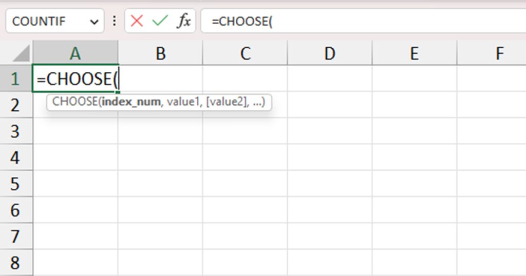
- index_num: the position of the value you wish to extract from the specified list.
- value: the list you want the function to extract from.
It is mandatory for you to insert the index_num and the first value in the CHOOSE function. You can add other values according to your convenience.
Additionally, you cannot pass a range as your list. You can pass a group of ranges when you’re nesting CHOOSE inside another function, however, you cannot pass one range to extract values from. This is because CHOOSE cannot locate your index_number from a range value.
Here are some of the ranges and the value they return when using the CHOOSE function.
| Formula | Result | Description |
| =CHOOSE(3, “Lilly”, “Rose”, “Tulip”) | Tulip | Returns the third text in the value section. |
| =CHOOSE(2, F2, F3, F4, F5, F6, F7, F8, F9, F10, F11) | Watermelon | Returns the cell content in cell F2. |
| =CHOOSE(11, F2, F3, F4, F5, F6, F7, F8, F9, F10, F11) | #VALUE! | There is no 11th value in the list. The index_num is out of range. |
| =CHOOSE(6, F2:F11) | #VALUE! | Can’t identify the sixth value from the specified list. |
How to Use CHOOSE Function in Excel
You can use CHOOSE as a lookup function, or nest the function with other functions to create a new condition to perform a certain calculation. Take a look at a couple of the examples we’ve listed below for a better understanding of the CHOOSE function in Excel.
Example 1: CHOOSE as a Lookup Function
You can use the CHOOSE function to simply extract a value from a list of values or cells.
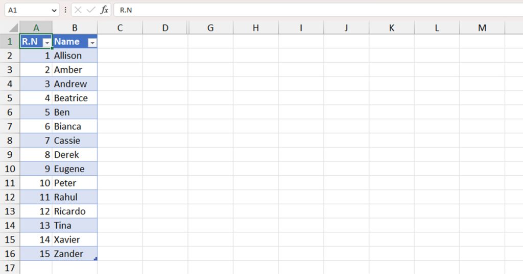
In this table, we have a list of names of 15 students according to their roll numbers. Take, for instance, you need to know the name of the student with roll number 7. You can put the list inside and command it to extract the 7th value from the list.
To make our formula a bit more dynamic, we entered the value “7” in cell F5. We will reference this cell in your formula in the index_col section. If we want to check out the names of other roll numbers in the future, we can simply change the value of F5 from 1-7.
Here’s how we constructed the CHOOSE function to extract the desired value:
=CHOOSE(F5, B2, B3, B4, B5, B6, B7, B8, B9, B10, B11, B12, B13, B14, B15, B16)
You can also use absolute referencing to lock in all of your cells.
Example 2: Nest CHOOSE Inside Another Function
The CHOOSE function works really well nested inside other functions. For this instance, let’s pair the CHOOSE function with the SUM function.
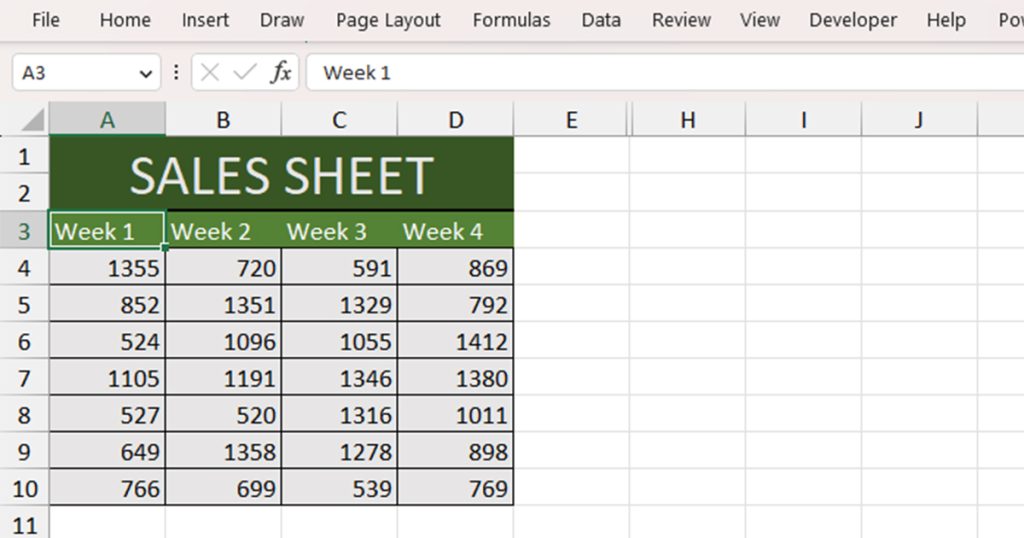
This data table has the sales sheet for each week for a month. We need to construct a formula where can view the sum of a set week from the list.
Like the previous method, we inserted the week number in a cell, in this case, cell G5to try and make our formula a bit more dynamic. We can change the number in this section to immediately change the week number we wish to generate the sum of.
Here is our formula:
=SUM(CHOOSE(G5,A4:A10,B4:B10,C4:C10,D4:D10))
Before you question the use of range in this formula, let me break the formula down for you. The ranges in this function act as individual list items. If the index_col is 3, it will call the third item from the list: C4:C10. As the SUM function takes in ranges as arguments, you will not get the #VALUE! error.
How to Avoid the #VALUE! Error While Using CHOOSE
By now, you could’ve guessed how easy it really is to stumble on the #VALUE! error when using the CHOOSE function. For starters, let’s assume that you shared a sheet with the second example with a peer. Instead of entering the index_col inside 1-4, they entered 7. As there really isn’t a 7th range from the value, you will encounter the #VALUE! Error.
My favorite tool to fool-proof mistakes as such is Data Validation.
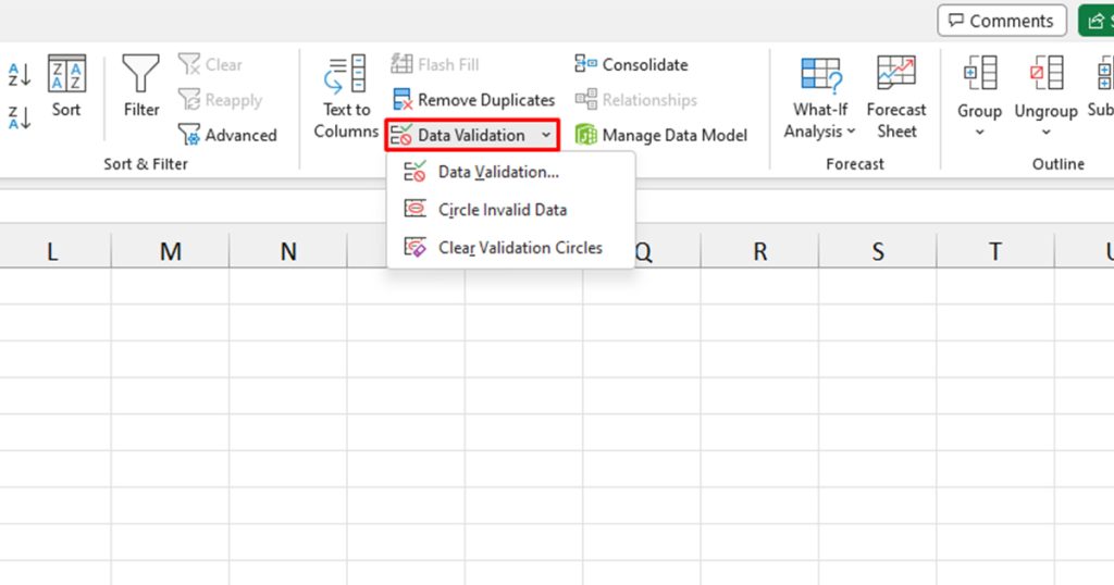
You can create a drop-down list to choose a value on the cell we referenced as the index_col. You can also go a step further by including an error message to instruct the user to enter a valid numeric value.